beginner/introyt/trainingyt

Run in Google Colab

Colab

Download Notebook

Notebook

View on GitHub

GitHub

Introduction || Tensors || Autograd || Building Models || TensorBoard Support || Training Models || Model Understanding

Training with PyTorch

Created On: Nov 30, 2021 | Last Updated: May 06, 2026 | Last Verified: Nov 05, 2024

Follow along with the video below or on youtube.

Introduction

In past videos, we’ve discussed and demonstrated:

• Building models with the neural network layers and functions of the torch.nn module

• The mechanics of automated gradient computation, which is central to gradient-based model training

• Using TensorBoard to visualize training progress and other activities

In this video, we’ll be adding some new tools to your inventory:

• We’ll get familiar with the dataset and dataloader abstractions, and how they ease the process of feeding data to your model during a training loop

• We’ll discuss specific loss functions and when to use them

• We’ll look at PyTorch optimizers, which implement algorithms to adjust model weights based on the outcome of a loss function

Finally, we’ll pull all of these together and see a full PyTorch training loop in action.

Dataset and DataLoader

The Dataset and DataLoader classes encapsulate the process of pulling your data from storage and exposing it to your training loop in batches.

The Dataset is responsible for accessing and processing single instances of data.

The DataLoader pulls instances of data from the Dataset (either automatically or with a sampler that you define), collects them in batches, and returns them for consumption by your training loop. The DataLoader works with all kinds of datasets, regardless of the type of data they contain.

For this tutorial, we’ll be using the Fashion-MNIST dataset provided by TorchVision. We use torchvision.transforms.v2.Normalize() to zero-center and normalize the distribution of the image tile content, and download both training and validation data splits.

import torch
import torchvision
from torchvision.transforms import v2

# PyTorch TensorBoard support
from torch.utils.tensorboard import SummaryWriter
from datetime import datetime


transform = v2.Compose([
    v2.ToImage(),
    v2.ToDtype(torch.float32, scale=True),
    v2.Normalize((0.5,), (0.5,))
])

# Create datasets for training & validation, download if necessary
training_set = torchvision.datasets.FashionMNIST('./data', train=True, transform=transform, download=True)
validation_set = torchvision.datasets.FashionMNIST('./data', train=False, transform=transform, download=True)

# Create data loaders for our datasets; shuffle for training, not for validation
training_loader = torch.utils.data.DataLoader(training_set, batch_size=4, shuffle=True)
validation_loader = torch.utils.data.DataLoader(validation_set, batch_size=4, shuffle=False)

# Class labels
classes = ('T-shirt/top', 'Trouser', 'Pullover', 'Dress', 'Coat',
        'Sandal', 'Shirt', 'Sneaker', 'Bag', 'Ankle Boot')

# Report split sizes
print(f'Training set has {len(training_set)} instances')
print(f'Validation set has {len(validation_set)} instances')

  0%|          | 0.00/26.4M [00:00<?, ?B/s]
  0%|          | 65.5k/26.4M [00:00<01:09, 378kB/s]
  1%|          | 229k/26.4M [00:00<00:36, 709kB/s]
  3%|▎         | 918k/26.4M [00:00<00:11, 2.19MB/s]
 14%|█▍        | 3.67M/26.4M [00:00<00:03, 7.55MB/s]
 37%|███▋      | 9.73M/26.4M [00:00<00:00, 17.4MB/s]
 60%|█████▉    | 15.8M/26.4M [00:01<00:00, 23.2MB/s]
 82%|████████▏ | 21.8M/26.4M [00:01<00:00, 26.9MB/s]
100%|██████████| 26.4M/26.4M [00:01<00:00, 20.1MB/s]

  0%|          | 0.00/29.5k [00:00<?, ?B/s]
100%|██████████| 29.5k/29.5k [00:00<00:00, 336kB/s]

  0%|          | 0.00/4.42M [00:00<?, ?B/s]
  1%|▏         | 65.5k/4.42M [00:00<00:11, 371kB/s]
  4%|▍         | 197k/4.42M [00:00<00:07, 590kB/s]
 18%|█▊        | 786k/4.42M [00:00<00:01, 1.85MB/s]
 70%|███████   | 3.11M/4.42M [00:00<00:00, 6.32MB/s]
100%|██████████| 4.42M/4.42M [00:00<00:00, 6.24MB/s]

  0%|          | 0.00/5.15k [00:00<?, ?B/s]
100%|██████████| 5.15k/5.15k [00:00<00:00, 49.4MB/s]
Training set has 60000 instances
Validation set has 10000 instances

As always, let’s visualize the data as a sanity check:

import matplotlib.pyplot as plt
import numpy as np

# Helper function for inline image display
def matplotlib_imshow(img, one_channel=False):
    if one_channel:
        img = img.mean(dim=0)
    img = img / 2 + 0.5     # unnormalize
    npimg = img.numpy()
    if one_channel:
        plt.imshow(npimg, cmap="Greys")
    else:
        plt.imshow(np.transpose(npimg, (1, 2, 0)))

dataiter = iter(training_loader)
images, labels = next(dataiter)

# Create a grid from the images and show them
img_grid = torchvision.utils.make_grid(images)
matplotlib_imshow(img_grid, one_channel=True)
print('  '.join(classes[labels[j]] for j in range(4)))

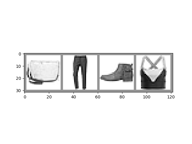
Ankle Boot  Pullover  T-shirt/top  Sneaker

The Model

The model we’ll use in this example is a variant of LeNet-5 - it should be familiar if you’ve watched the previous videos in this series.

import torch.nn as nn
import torch.nn.functional as F

# PyTorch models inherit from torch.nn.Module
class GarmentClassifier(nn.Module):
    def __init__(self):
        super().__init__()
        self.conv1 = nn.Conv2d(1, 6, 5)
        self.pool = nn.MaxPool2d(2, 2)
        self.conv2 = nn.Conv2d(6, 16, 5)
        self.fc1 = nn.Linear(16 * 4 * 4, 120)
        self.fc2 = nn.Linear(120, 84)
        self.fc3 = nn.Linear(84, 10)

    def forward(self, x):
        x = self.pool(F.relu(self.conv1(x)))
        x = self.pool(F.relu(self.conv2(x)))
        x = x.view(-1, 16 * 4 * 4)
        x = F.relu(self.fc1(x))
        x = F.relu(self.fc2(x))
        x = self.fc3(x)
        return x


model = GarmentClassifier()

Loss Function

For this example, we’ll be using a cross-entropy loss. For demonstration purposes, we’ll create batches of dummy output and label values, run them through the loss function, and examine the result.

loss_fn = torch.nn.CrossEntropyLoss()

# NB: Loss functions expect data in batches, so we're creating batches of 4
# Represents the model's confidence in each of the 10 classes for a given input
dummy_outputs = torch.rand(4, 10)
# Represents the correct class among the 10 being tested
dummy_labels = torch.tensor([1, 5, 3, 7])

print(dummy_outputs)
print(dummy_labels)

loss = loss_fn(dummy_outputs, dummy_labels)
print(f'Total loss for this batch: {loss.item()}')

tensor([[0.4008, 0.4060, 0.4004, 0.9502, 0.0278, 0.4385, 0.2489, 0.6035, 0.8319,
         0.8243],
        [0.2132, 0.3977, 0.7193, 0.1888, 0.5707, 0.2165, 0.2616, 0.5768, 0.4650,
         0.1168],
        [0.5506, 0.8866, 0.6000, 0.8737, 0.8739, 0.7224, 0.7166, 0.8803, 0.8337,
         0.1427],
        [0.2248, 0.5781, 0.8963, 0.1595, 0.2728, 0.4167, 0.8045, 0.5442, 0.6149,
         0.9415]])
tensor([1, 5, 3, 7])
Total loss for this batch: 2.3554961681365967

Optimizer

For this example, we’ll be using simple stochastic gradient descent with momentum.

It can be instructive to try some variations on this optimization scheme:

• Learning rate determines the size of the steps the optimizer takes. What does a different learning rate do to the your training results, in terms of accuracy and convergence time?

• Momentum nudges the optimizer in the direction of strongest gradient over multiple steps. What does changing this value do to your results?

• Try some different optimization algorithms, such as averaged SGD, Adagrad, or Adam. How do your results differ?

# Optimizers specified in the torch.optim package
optimizer = torch.optim.SGD(model.parameters(), lr=0.001, momentum=0.9)

The Training Loop

Below, we have a function that performs one training epoch. It enumerates data from the DataLoader, and on each pass of the loop does the following:

• Gets a batch of training data from the DataLoader

• Zeros the optimizer’s gradients

• Performs an inference - that is, gets predictions from the model for an input batch

• Calculates the loss for that set of predictions vs. the labels on the dataset

• Calculates the backward gradients over the learning weights

• Tells the optimizer to perform one learning step - that is, adjust the model’s learning weights based on the observed gradients for this batch, according to the optimization algorithm we chose

• It reports on the loss for every 1000 batches.

• Finally, it reports the average per-batch loss for the last 1000 batches, for comparison with a validation run

def train_one_epoch(epoch_index, tb_writer):
    running_loss = 0.
    last_loss = 0.

    # Here, we use enumerate(training_loader) instead of
    # iter(training_loader) so that we can track the batch
    # index and do some intra-epoch reporting
    for i, data in enumerate(training_loader):
        # Every data instance is an input + label pair
        inputs, labels = data

        # Zero your gradients for every batch!
        optimizer.zero_grad()

        # Make predictions for this batch
        outputs = model(inputs)

        # Compute the loss and its gradients
        loss = loss_fn(outputs, labels)
        loss.backward()

        # Adjust learning weights
        optimizer.step()

        # Gather data and report
        running_loss += loss.item()
        if i % 1000 == 999:
            last_loss = running_loss / 1000 # loss per batch
            print(f'  batch {i + 1} loss: {last_loss}')
            tb_x = epoch_index * len(training_loader) + i + 1
            tb_writer.add_scalar('Loss/train', last_loss, tb_x)
            running_loss = 0.

    return last_loss

Per-Epoch Activity

There are a couple of things we’ll want to do once per epoch:

• Perform validation by checking our relative loss on a set of data that was not used for training, and report this

• Save a copy of the model

Here, we’ll do our reporting in TensorBoard. This will require going to the command line to start TensorBoard, and opening it in another browser tab.

# Initializing in a separate cell so we can easily add more epochs to the same run
timestamp = datetime.now().strftime('%Y%m%d_%H%M%S')
writer = SummaryWriter(f'runs/fashion_trainer_{timestamp}')
epoch_number = 0

EPOCHS = 5

best_vloss = 1_000_000.

for epoch in range(EPOCHS):
    print(f'EPOCH {epoch_number + 1}:')

    # Make sure gradient tracking is on, and do a pass over the data
    model.train(True)
    avg_loss = train_one_epoch(epoch_number, writer)


    running_vloss = 0.0
    # Set the model to evaluation mode, disabling dropout and using population
    # statistics for batch normalization.
    model.eval()

    # Disable gradient computation and reduce memory consumption.
    with torch.no_grad():
        for i, vdata in enumerate(validation_loader):
            vinputs, vlabels = vdata
            voutputs = model(vinputs)
            vloss = loss_fn(voutputs, vlabels)
            running_vloss += vloss

    avg_vloss = running_vloss / (i + 1)
    print(f'LOSS train {avg_loss} valid {avg_vloss}')

    # Log the running loss averaged per batch
    # for both training and validation
    writer.add_scalars('Training vs. Validation Loss',
                    { 'Training' : avg_loss, 'Validation' : avg_vloss },
                    epoch_number + 1)
    writer.flush()

    # Track best performance, and save the model's state
    if avg_vloss < best_vloss:
        best_vloss = avg_vloss
        model_path = f'model_{timestamp}_{epoch_number}'
        torch.save(model.state_dict(), model_path)

    epoch_number += 1

EPOCH 1:
  batch 1000 loss: 1.6490134096890687
  batch 2000 loss: 0.8794220873713493
  batch 3000 loss: 0.6920068377633579
  batch 4000 loss: 0.6548182668378577
  batch 5000 loss: 0.6056985420037526
  batch 6000 loss: 0.564624475349905
  batch 7000 loss: 0.5399795940891199
  batch 8000 loss: 0.5364603952636826
  batch 9000 loss: 0.503451196585549
  batch 10000 loss: 0.491504361334024
  batch 11000 loss: 0.477360519093927
  batch 12000 loss: 0.46786118267592974
  batch 13000 loss: 0.4438537150732591
  batch 14000 loss: 0.435872395854909
  batch 15000 loss: 0.42765479374787535
LOSS train 0.42765479374787535 valid 0.44690054655075073
EPOCH 2:
  batch 1000 loss: 0.4162398645043722
  batch 2000 loss: 0.41995261479506735
  batch 3000 loss: 0.4172815731718438
  batch 4000 loss: 0.36986394727887817
  batch 5000 loss: 0.38002498116352945
  batch 6000 loss: 0.389014043433679
  batch 7000 loss: 0.3778508409477654
  batch 8000 loss: 0.3960505936787813
  batch 9000 loss: 0.3656966466306767
  batch 10000 loss: 0.3688230440270272
  batch 11000 loss: 0.36166456335978
  batch 12000 loss: 0.36258256799264926
  batch 13000 loss: 0.35431309579184744
  batch 14000 loss: 0.34879590120259674
  batch 15000 loss: 0.3644959595497057
LOSS train 0.3644959595497057 valid 0.36823609471321106
EPOCH 3:
  batch 1000 loss: 0.34044388455350416
  batch 2000 loss: 0.32436358434688006
  batch 3000 loss: 0.33842317014344736
  batch 4000 loss: 0.3364472628404619
  batch 5000 loss: 0.32447360131682945
  batch 6000 loss: 0.31102842848727597
  batch 7000 loss: 0.33485471606998907
  batch 8000 loss: 0.3293339918176789
  batch 9000 loss: 0.34065036369790325
  batch 10000 loss: 0.3262448830557787
  batch 11000 loss: 0.3372839359218087
  batch 12000 loss: 0.3351387796745621
  batch 13000 loss: 0.33495071126852416
  batch 14000 loss: 0.31444868071567905
  batch 15000 loss: 0.3173477705280529
LOSS train 0.3173477705280529 valid 0.3291745185852051
EPOCH 4:
  batch 1000 loss: 0.2974653250033007
  batch 2000 loss: 0.33536598401011725
  batch 3000 loss: 0.2806962358472083
  batch 4000 loss: 0.3098943673290196
  batch 5000 loss: 0.3236401898502518
  batch 6000 loss: 0.3011308161323177
  batch 7000 loss: 0.31380102527805137
  batch 8000 loss: 0.3139864266534187
  batch 9000 loss: 0.31926461398215905
  batch 10000 loss: 0.2811458704107245
  batch 11000 loss: 0.3035927659050212
  batch 12000 loss: 0.3008047970955959
  batch 13000 loss: 0.30102620854483847
  batch 14000 loss: 0.2856070303207816
  batch 15000 loss: 0.31378861948487613
LOSS train 0.31378861948487613 valid 0.32736483216285706
EPOCH 5:
  batch 1000 loss: 0.28168964856820095
  batch 2000 loss: 0.27313915011458084
  batch 3000 loss: 0.29790957588958555
  batch 4000 loss: 0.30495057670990355
  batch 5000 loss: 0.2914723885890453
  batch 6000 loss: 0.2700535023240573
  batch 7000 loss: 0.3010115914536291
  batch 8000 loss: 0.2852006104638349
  batch 9000 loss: 0.286087478606617
  batch 10000 loss: 0.29179737023318014
  batch 11000 loss: 0.2830669925537659
  batch 12000 loss: 0.27302959646120145
  batch 13000 loss: 0.2904240637791245
  batch 14000 loss: 0.3009752814811618
  batch 15000 loss: 0.29678103559796
LOSS train 0.29678103559796 valid 0.31956714391708374

To load a saved version of the model:

saved_model = GarmentClassifier()
saved_model.load_state_dict(torch.load(PATH))

Once you’ve loaded the model, it’s ready for whatever you need it for - more training, inference, or analysis.

Note that if your model has constructor parameters that affect model structure, you’ll need to provide them and configure the model identically to the state in which it was saved.

Other Resources

• Docs on the data utilities, including Dataset and DataLoader, at pytorch.org

• A note on the use of pinned memory for GPU training

• Documentation on the datasets available in TorchVision, TorchText, and TorchAudio

• Documentation on the loss functions available in PyTorch

• Documentation on the torch.optim package, which includes optimizers and related tools, such as learning rate scheduling

• A detailed tutorial on saving and loading models

• The Tutorials section of pytorch.org contains tutorials on a broad variety of training tasks, including classification in different domains, generative adversarial networks, reinforcement learning, and more