



Note
Go to the end to download the full example code.
Transfer Learning for Computer Vision Tutorial#
Created On: Mar 24, 2017 | Last Updated: Jan 27, 2025 | Last Verified: Nov 05, 2024
Author: Sasank Chilamkurthy
In this tutorial, you will learn how to train a convolutional neural network for image classification using transfer learning. You can read more about the transfer learning at cs231n notes
Quoting these notes,
In practice, very few people train an entire Convolutional Network from scratch (with random initialization), because it is relatively rare to have a dataset of sufficient size. Instead, it is common to pretrain a ConvNet on a very large dataset (e.g. ImageNet, which contains 1.2 million images with 1000 categories), and then use the ConvNet either as an initialization or a fixed feature extractor for the task of interest.
These two major transfer learning scenarios look as follows:
Finetuning the ConvNet: Instead of random initialization, we initialize the network with a pretrained network, like the one that is trained on imagenet 1000 dataset. Rest of the training looks as usual.
ConvNet as fixed feature extractor: Here, we will freeze the weights for all of the network except that of the final fully connected layer. This last fully connected layer is replaced with a new one with random weights and only this layer is trained.
# License: BSD
# Author: Sasank Chilamkurthy

import torch
import torch.nn as nn
import torch.optim as optim
from torch.optim import lr_scheduler
import torch.backends.cudnn as cudnn
import numpy as np
import torchvision
from torchvision import datasets, models, transforms
import matplotlib.pyplot as plt
import time
import os
from PIL import Image
from tempfile import TemporaryDirectory

cudnn.benchmark = True
plt.ion()   # interactive mode
<contextlib.ExitStack object at 0x7f5fc1026a10>
Load Data#
We will use torchvision and torch.utils.data packages for loading the data.
The problem we’re going to solve today is to train a model to classify ants and bees. We have about 120 training images each for ants and bees. There are 75 validation images for each class. Usually, this is a very small dataset to generalize upon, if trained from scratch. Since we are using transfer learning, we should be able to generalize reasonably well.
This dataset is a very small subset of imagenet.
Note
Download the data from here and extract it to the current directory.
# Data augmentation and normalization for training
# Just normalization for validation
data_transforms = {
    'train': transforms.Compose([
        transforms.RandomResizedCrop(224),
        transforms.RandomHorizontalFlip(),
        transforms.ToTensor(),
        transforms.Normalize([0.485, 0.456, 0.406], [0.229, 0.224, 0.225])
    ]),
    'val': transforms.Compose([
        transforms.Resize(256),
        transforms.CenterCrop(224),
        transforms.ToTensor(),
        transforms.Normalize([0.485, 0.456, 0.406], [0.229, 0.224, 0.225])
    ]),
}

data_dir = 'data/hymenoptera_data'
image_datasets = {x: datasets.ImageFolder(os.path.join(data_dir, x),
                                          data_transforms[x])
                  for x in ['train', 'val']}
dataloaders = {x: torch.utils.data.DataLoader(image_datasets[x], batch_size=4,
                                             shuffle=True, num_workers=4)
              for x in ['train', 'val']}
dataset_sizes = {x: len(image_datasets[x]) for x in ['train', 'val']}
class_names = image_datasets['train'].classes

# We want to be able to train our model on an `accelerator <https://pytorch.org/docs/stable/torch.html#accelerators>`__
# such as CUDA, MPS, MTIA, or XPU. If the current accelerator is available, we will use it. Otherwise, we use the CPU.

device = torch.accelerator.current_accelerator().type if torch.accelerator.is_available() else "cpu"
print(f"Using {device} device")
Using cuda device
Visualize a few images#
Let’s visualize a few training images so as to understand the data augmentations.
def imshow(inp, title=None):
    """Display image for Tensor."""
    inp = inp.numpy().transpose((1, 2, 0))
    mean = np.array([0.485, 0.456, 0.406])
    std = np.array([0.229, 0.224, 0.225])
    inp = std * inp + mean
    inp = np.clip(inp, 0, 1)
    plt.imshow(inp)
    if title is not None:
        plt.title(title)
    plt.pause(0.001)  # pause a bit so that plots are updated


# Get a batch of training data
inputs, classes = next(iter(dataloaders['train']))

# Make a grid from batch
out = torchvision.utils.make_grid(inputs)

imshow(out, title=[class_names[x] for x in classes])
![['bees', 'ants', 'ants', 'bees']](../_images/sphx_glr_transfer_learning_tutorial_001.png)
Training the model#
Now, let’s write a general function to train a model. Here, we will illustrate:
Scheduling the learning rate
Saving the best model
In the following, parameter scheduler is an LR scheduler object from
torch.optim.lr_scheduler.
def train_model(model, criterion, optimizer, scheduler, num_epochs=25):
    since = time.time()

    # Create a temporary directory to save training checkpoints
    with TemporaryDirectory() as tempdir:
        best_model_params_path = os.path.join(tempdir, 'best_model_params.pt')

        torch.save(model.state_dict(), best_model_params_path)
        best_acc = 0.0

        for epoch in range(num_epochs):
            print(f'Epoch {epoch}/{num_epochs - 1}')
            print('-' * 10)

            # Each epoch has a training and validation phase
            for phase in ['train', 'val']:
                if phase == 'train':
                    model.train()  # Set model to training mode
                else:
                    model.eval()   # Set model to evaluate mode

                running_loss = 0.0
                running_corrects = 0

                # Iterate over data.
                for inputs, labels in dataloaders[phase]:
                    inputs = inputs.to(device)
                    labels = labels.to(device)

                    # zero the parameter gradients
                    optimizer.zero_grad()

                    # forward
                    # track history if only in train
                    with torch.set_grad_enabled(phase == 'train'):
                        outputs = model(inputs)
                        _, preds = torch.max(outputs, 1)
                        loss = criterion(outputs, labels)

                        # backward + optimize only if in training phase
                        if phase == 'train':
                            loss.backward()
                            optimizer.step()

                    # statistics
                    running_loss += loss.item() * inputs.size(0)
                    running_corrects += torch.sum(preds == labels.data)
                if phase == 'train':
                    scheduler.step()

                epoch_loss = running_loss / dataset_sizes[phase]
                epoch_acc = running_corrects.double() / dataset_sizes[phase]

                print(f'{phase} Loss: {epoch_loss:.4f} Acc: {epoch_acc:.4f}')

                # deep copy the model
                if phase == 'val' and epoch_acc > best_acc:
                    best_acc = epoch_acc
                    torch.save(model.state_dict(), best_model_params_path)

            print()

        time_elapsed = time.time() - since
        print(f'Training complete in {time_elapsed // 60:.0f}m {time_elapsed % 60:.0f}s')
        print(f'Best val Acc: {best_acc:4f}')

        # load best model weights
        model.load_state_dict(torch.load(best_model_params_path, weights_only=True))
    return model
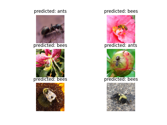
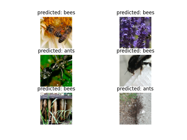
Visualizing the model predictions#
Generic function to display predictions for a few images
def visualize_model(model, num_images=6):
    was_training = model.training
    model.eval()
    images_so_far = 0
    fig = plt.figure()

    with torch.no_grad():
        for i, (inputs, labels) in enumerate(dataloaders['val']):
            inputs = inputs.to(device)
            labels = labels.to(device)

            outputs = model(inputs)
            _, preds = torch.max(outputs, 1)

            for j in range(inputs.size()[0]):
                images_so_far += 1
                ax = plt.subplot(num_images//2, 2, images_so_far)
                ax.axis('off')
                ax.set_title(f'predicted: {class_names[preds[j]]}')
                imshow(inputs.cpu().data[j])

                if images_so_far == num_images:
                    model.train(mode=was_training)
                    return
        model.train(mode=was_training)
Finetuning the ConvNet#
Load a pretrained model and reset final fully connected layer.
model_ft = models.resnet18(weights='IMAGENET1K_V1')
num_ftrs = model_ft.fc.in_features
# Here the size of each output sample is set to 2.
# Alternatively, it can be generalized to ``nn.Linear(num_ftrs, len(class_names))``.
model_ft.fc = nn.Linear(num_ftrs, 2)

model_ft = model_ft.to(device)

criterion = nn.CrossEntropyLoss()

# Observe that all parameters are being optimized
optimizer_ft = optim.SGD(model_ft.parameters(), lr=0.001, momentum=0.9)

# Decay LR by a factor of 0.1 every 7 epochs
exp_lr_scheduler = lr_scheduler.StepLR(optimizer_ft, step_size=7, gamma=0.1)
Downloading: "https://download.pytorch.org/models/resnet18-f37072fd.pth" to /var/lib/ci-user/.cache/torch/hub/checkpoints/resnet18-f37072fd.pth

  0%|          | 0.00/44.7M [00:00<?, ?B/s]
 93%|█████████▎| 41.6M/44.7M [00:00<00:00, 436MB/s]
100%|██████████| 44.7M/44.7M [00:00<00:00, 436MB/s]
Train and evaluate#
It should take around 15-25 min on CPU. On GPU though, it takes less than a minute.
model_ft = train_model(model_ft, criterion, optimizer_ft, exp_lr_scheduler,
                       num_epochs=25)
Epoch 0/24
----------
train Loss: 0.6612 Acc: 0.6803
val Loss: 0.1409 Acc: 0.9477

Epoch 1/24
----------
train Loss: 0.4755 Acc: 0.7828
val Loss: 0.2146 Acc: 0.9150

Epoch 2/24
----------
train Loss: 0.5166 Acc: 0.7746
val Loss: 0.2666 Acc: 0.9281

Epoch 3/24
----------
train Loss: 0.5501 Acc: 0.7500
val Loss: 0.2341 Acc: 0.9150

Epoch 4/24
----------
train Loss: 0.5132 Acc: 0.7828
val Loss: 0.1981 Acc: 0.9150

Epoch 5/24
----------
train Loss: 0.4480 Acc: 0.8320
val Loss: 0.3568 Acc: 0.8889

Epoch 6/24
----------
train Loss: 0.3836 Acc: 0.8484
val Loss: 0.3188 Acc: 0.9216

Epoch 7/24
----------
train Loss: 0.4447 Acc: 0.8361
val Loss: 0.2229 Acc: 0.9346

Epoch 8/24
----------
train Loss: 0.3733 Acc: 0.8320
val Loss: 0.2271 Acc: 0.9346

Epoch 9/24
----------
train Loss: 0.3634 Acc: 0.8238
val Loss: 0.1876 Acc: 0.9412

Epoch 10/24
----------
train Loss: 0.2330 Acc: 0.8975
val Loss: 0.2104 Acc: 0.9085

Epoch 11/24
----------
train Loss: 0.3573 Acc: 0.8443
val Loss: 0.1940 Acc: 0.9281

Epoch 12/24
----------
train Loss: 0.2545 Acc: 0.8934
val Loss: 0.1862 Acc: 0.9412

Epoch 13/24
----------
train Loss: 0.3195 Acc: 0.8525
val Loss: 0.1754 Acc: 0.9412

Epoch 14/24
----------
train Loss: 0.2098 Acc: 0.9057
val Loss: 0.1786 Acc: 0.9412

Epoch 15/24
----------
train Loss: 0.2558 Acc: 0.8975
val Loss: 0.1759 Acc: 0.9477

Epoch 16/24
----------
train Loss: 0.2772 Acc: 0.8975
val Loss: 0.1724 Acc: 0.9412

Epoch 17/24
----------
train Loss: 0.3179 Acc: 0.8525
val Loss: 0.1743 Acc: 0.9412

Epoch 18/24
----------
train Loss: 0.3337 Acc: 0.8730
val Loss: 0.1724 Acc: 0.9477

Epoch 19/24
----------
train Loss: 0.2996 Acc: 0.8852
val Loss: 0.1661 Acc: 0.9412

Epoch 20/24
----------
train Loss: 0.2194 Acc: 0.9057
val Loss: 0.1798 Acc: 0.9412

Epoch 21/24
----------
train Loss: 0.2800 Acc: 0.8975
val Loss: 0.1808 Acc: 0.9477

Epoch 22/24
----------
train Loss: 0.2486 Acc: 0.9057
val Loss: 0.1545 Acc: 0.9412

Epoch 23/24
----------
train Loss: 0.2087 Acc: 0.9057
val Loss: 0.1766 Acc: 0.9412

Epoch 24/24
----------
train Loss: 0.2730 Acc: 0.8811
val Loss: 0.1799 Acc: 0.9412

Training complete in 0m 36s
Best val Acc: 0.947712
visualize_model(model_ft)
ConvNet as fixed feature extractor#
Here, we need to freeze all the network except the final layer. We need
to set requires_grad = False to freeze the parameters so that the
gradients are not computed in backward().
You can read more about this in the documentation here.
model_conv = torchvision.models.resnet18(weights='IMAGENET1K_V1')
for param in model_conv.parameters():
    param.requires_grad = False

# Parameters of newly constructed modules have requires_grad=True by default
num_ftrs = model_conv.fc.in_features
model_conv.fc = nn.Linear(num_ftrs, 2)

model_conv = model_conv.to(device)

criterion = nn.CrossEntropyLoss()

# Observe that only parameters of final layer are being optimized as
# opposed to before.
optimizer_conv = optim.SGD(model_conv.fc.parameters(), lr=0.001, momentum=0.9)

# Decay LR by a factor of 0.1 every 7 epochs
exp_lr_scheduler = lr_scheduler.StepLR(optimizer_conv, step_size=7, gamma=0.1)
Train and evaluate#
On CPU this will take about half the time compared to previous scenario. This is expected as gradients don’t need to be computed for most of the network. However, forward does need to be computed.
model_conv = train_model(model_conv, criterion, optimizer_conv,
                         exp_lr_scheduler, num_epochs=25)
Epoch 0/24
----------
train Loss: 0.7171 Acc: 0.6107
val Loss: 0.2107 Acc: 0.9412

Epoch 1/24
----------
train Loss: 0.5086 Acc: 0.7746
val Loss: 0.7011 Acc: 0.7124

Epoch 2/24
----------
train Loss: 0.5736 Acc: 0.7705
val Loss: 0.2882 Acc: 0.8889

Epoch 3/24
----------
train Loss: 0.4581 Acc: 0.8074
val Loss: 0.2848 Acc: 0.8824

Epoch 4/24
----------
train Loss: 0.4921 Acc: 0.7828
val Loss: 0.4383 Acc: 0.8301

Epoch 5/24
----------
train Loss: 0.5450 Acc: 0.7541
val Loss: 0.2217 Acc: 0.9150

Epoch 6/24
----------
train Loss: 0.4649 Acc: 0.8156
val Loss: 0.5898 Acc: 0.7974

Epoch 7/24
----------
train Loss: 0.4186 Acc: 0.8402
val Loss: 0.1664 Acc: 0.9608

Epoch 8/24
----------
train Loss: 0.3546 Acc: 0.8402
val Loss: 0.1787 Acc: 0.9608

Epoch 9/24
----------
train Loss: 0.2828 Acc: 0.8525
val Loss: 0.1677 Acc: 0.9477

Epoch 10/24
----------
train Loss: 0.2564 Acc: 0.8730
val Loss: 0.1851 Acc: 0.9608

Epoch 11/24
----------
train Loss: 0.4187 Acc: 0.8279
val Loss: 0.1802 Acc: 0.9608

Epoch 12/24
----------
train Loss: 0.3101 Acc: 0.8770
val Loss: 0.1693 Acc: 0.9477

Epoch 13/24
----------
train Loss: 0.2941 Acc: 0.8852
val Loss: 0.1618 Acc: 0.9608

Epoch 14/24
----------
train Loss: 0.3829 Acc: 0.8279
val Loss: 0.1873 Acc: 0.9608

Epoch 15/24
----------
train Loss: 0.2944 Acc: 0.8648
val Loss: 0.1729 Acc: 0.9608

Epoch 16/24
----------
train Loss: 0.4055 Acc: 0.8033
val Loss: 0.1616 Acc: 0.9608

Epoch 17/24
----------
train Loss: 0.4019 Acc: 0.8320
val Loss: 0.1986 Acc: 0.9542

Epoch 18/24
----------
train Loss: 0.2956 Acc: 0.8689
val Loss: 0.1898 Acc: 0.9608

Epoch 19/24
----------
train Loss: 0.3104 Acc: 0.8648
val Loss: 0.1665 Acc: 0.9608

Epoch 20/24
----------
train Loss: 0.3875 Acc: 0.8484
val Loss: 0.1801 Acc: 0.9608

Epoch 21/24
----------
train Loss: 0.3413 Acc: 0.8402
val Loss: 0.1828 Acc: 0.9608

Epoch 22/24
----------
train Loss: 0.3152 Acc: 0.8770
val Loss: 0.1845 Acc: 0.9608

Epoch 23/24
----------
train Loss: 0.3338 Acc: 0.8770
val Loss: 0.1875 Acc: 0.9542

Epoch 24/24
----------
train Loss: 0.3448 Acc: 0.8238
val Loss: 0.1838 Acc: 0.9608

Training complete in 0m 27s
Best val Acc: 0.960784
visualize_model(model_conv)

plt.ioff()
plt.show()
Inference on custom images#
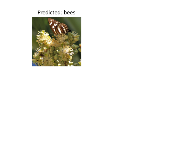
Use the trained model to make predictions on custom images and visualize the predicted class labels along with the images.
def visualize_model_predictions(model,img_path):
    was_training = model.training
    model.eval()

    img = Image.open(img_path)
    img = data_transforms['val'](img)
    img = img.unsqueeze(0)
    img = img.to(device)

    with torch.no_grad():
        outputs = model(img)
        _, preds = torch.max(outputs, 1)

        ax = plt.subplot(2,2,1)
        ax.axis('off')
        ax.set_title(f'Predicted: {class_names[preds[0]]}')
        imshow(img.cpu().data[0])

        model.train(mode=was_training)
visualize_model_predictions(
    model_conv,
    img_path='data/hymenoptera_data/val/bees/72100438_73de9f17af.jpg'
)

plt.ioff()
plt.show()
Further Learning#
If you would like to learn more about the applications of transfer learning, checkout our Quantized Transfer Learning for Computer Vision Tutorial.
Total running time of the script: (1 minutes 5.676 seconds)