


Note
Go to the end to download the full example code.
Introduction || Tensors || Autograd || Building Models || TensorBoard Support || Training Models || Model Understanding
Training with PyTorch#
Created On: Nov 30, 2021 | Last Updated: May 06, 2026 | Last Verified: Nov 05, 2024
Follow along with the video below or on youtube.
Introduction#
In past videos, we’ve discussed and demonstrated:
Building models with the neural network layers and functions of the torch.nn module
The mechanics of automated gradient computation, which is central to gradient-based model training
Using TensorBoard to visualize training progress and other activities
In this video, we’ll be adding some new tools to your inventory:
We’ll get familiar with the dataset and dataloader abstractions, and how they ease the process of feeding data to your model during a training loop
We’ll discuss specific loss functions and when to use them
We’ll look at PyTorch optimizers, which implement algorithms to adjust model weights based on the outcome of a loss function
Finally, we’ll pull all of these together and see a full PyTorch training loop in action.
Dataset and DataLoader#
The Dataset and DataLoader classes encapsulate the process of
pulling your data from storage and exposing it to your training loop in
batches.
The Dataset is responsible for accessing and processing single
instances of data.
The DataLoader pulls instances of data from the Dataset (either
automatically or with a sampler that you define), collects them in
batches, and returns them for consumption by your training loop. The
DataLoader works with all kinds of datasets, regardless of the type
of data they contain.
For this tutorial, we’ll be using the Fashion-MNIST dataset provided by
TorchVision. We use torchvision.transforms.v2.Normalize() to
zero-center and normalize the distribution of the image tile content,
and download both training and validation data splits.
import torch
import torchvision
from torchvision.transforms import v2

# PyTorch TensorBoard support
from torch.utils.tensorboard import SummaryWriter
from datetime import datetime


transform = v2.Compose([
    v2.ToImage(),
    v2.ToDtype(torch.float32, scale=True),
    v2.Normalize((0.5,), (0.5,))
])

# Create datasets for training & validation, download if necessary
training_set = torchvision.datasets.FashionMNIST('./data', train=True, transform=transform, download=True)
validation_set = torchvision.datasets.FashionMNIST('./data', train=False, transform=transform, download=True)

# Create data loaders for our datasets; shuffle for training, not for validation
training_loader = torch.utils.data.DataLoader(training_set, batch_size=4, shuffle=True)
validation_loader = torch.utils.data.DataLoader(validation_set, batch_size=4, shuffle=False)

# Class labels
classes = ('T-shirt/top', 'Trouser', 'Pullover', 'Dress', 'Coat',
        'Sandal', 'Shirt', 'Sneaker', 'Bag', 'Ankle Boot')

# Report split sizes
print(f'Training set has {len(training_set)} instances')
print(f'Validation set has {len(validation_set)} instances')
  0%|          | 0.00/26.4M [00:00<?, ?B/s]
  0%|          | 65.5k/26.4M [00:00<01:10, 373kB/s]
  1%|          | 229k/26.4M [00:00<00:37, 700kB/s]
  3%|▎         | 918k/26.4M [00:00<00:11, 2.16MB/s]
 14%|█▍        | 3.67M/26.4M [00:00<00:03, 7.45MB/s]
 37%|███▋      | 9.80M/26.4M [00:00<00:00, 17.3MB/s]
 61%|██████    | 16.0M/26.4M [00:01<00:00, 23.3MB/s]
 84%|████████▍ | 22.2M/26.4M [00:01<00:00, 27.1MB/s]
100%|██████████| 26.4M/26.4M [00:01<00:00, 19.8MB/s]

  0%|          | 0.00/29.5k [00:00<?, ?B/s]
100%|██████████| 29.5k/29.5k [00:00<00:00, 338kB/s]

  0%|          | 0.00/4.42M [00:00<?, ?B/s]
  1%|▏         | 65.5k/4.42M [00:00<00:11, 375kB/s]
  5%|▌         | 229k/4.42M [00:00<00:05, 706kB/s]
 21%|██        | 918k/4.42M [00:00<00:01, 2.18MB/s]
 82%|████████▏ | 3.64M/4.42M [00:00<00:00, 8.25MB/s]
100%|██████████| 4.42M/4.42M [00:00<00:00, 6.31MB/s]

  0%|          | 0.00/5.15k [00:00<?, ?B/s]
100%|██████████| 5.15k/5.15k [00:00<00:00, 58.7MB/s]
Training set has 60000 instances
Validation set has 10000 instances
As always, let’s visualize the data as a sanity check:
import matplotlib.pyplot as plt
import numpy as np

# Helper function for inline image display
def matplotlib_imshow(img, one_channel=False):
    if one_channel:
        img = img.mean(dim=0)
    img = img / 2 + 0.5     # unnormalize
    npimg = img.numpy()
    if one_channel:
        plt.imshow(npimg, cmap="Greys")
    else:
        plt.imshow(np.transpose(npimg, (1, 2, 0)))

dataiter = iter(training_loader)
images, labels = next(dataiter)

# Create a grid from the images and show them
img_grid = torchvision.utils.make_grid(images)
matplotlib_imshow(img_grid, one_channel=True)
print('  '.join(classes[labels[j]] for j in range(4)))
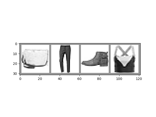
Sandal Dress T-shirt/top Dress
The Model#
The model we’ll use in this example is a variant of LeNet-5 - it should be familiar if you’ve watched the previous videos in this series.
import torch.nn as nn
import torch.nn.functional as F

# PyTorch models inherit from torch.nn.Module
class GarmentClassifier(nn.Module):
    def __init__(self):
        super().__init__()
        self.conv1 = nn.Conv2d(1, 6, 5)
        self.pool = nn.MaxPool2d(2, 2)
        self.conv2 = nn.Conv2d(6, 16, 5)
        self.fc1 = nn.Linear(16 * 4 * 4, 120)
        self.fc2 = nn.Linear(120, 84)
        self.fc3 = nn.Linear(84, 10)

    def forward(self, x):
        x = self.pool(F.relu(self.conv1(x)))
        x = self.pool(F.relu(self.conv2(x)))
        x = x.view(-1, 16 * 4 * 4)
        x = F.relu(self.fc1(x))
        x = F.relu(self.fc2(x))
        x = self.fc3(x)
        return x


model = GarmentClassifier()
Loss Function#
For this example, we’ll be using a cross-entropy loss. For demonstration purposes, we’ll create batches of dummy output and label values, run them through the loss function, and examine the result.
loss_fn = torch.nn.CrossEntropyLoss()

# NB: Loss functions expect data in batches, so we're creating batches of 4
# Represents the model's confidence in each of the 10 classes for a given input
dummy_outputs = torch.rand(4, 10)
# Represents the correct class among the 10 being tested
dummy_labels = torch.tensor([1, 5, 3, 7])

print(dummy_outputs)
print(dummy_labels)

loss = loss_fn(dummy_outputs, dummy_labels)
print(f'Total loss for this batch: {loss.item()}')
tensor([[8.7108e-01, 7.9464e-01, 8.5520e-01, 9.4068e-01, 5.0302e-01, 9.6517e-01,
         5.3978e-04, 4.8035e-01, 9.8412e-01, 4.2225e-01],
        [4.0291e-01, 4.5843e-01, 3.7892e-01, 8.0920e-01, 9.0322e-01, 1.9510e-01,
         7.2442e-01, 7.1048e-01, 2.0796e-01, 8.6231e-01],
        [5.3401e-01, 6.8077e-01, 6.4725e-01, 7.2985e-01, 9.2879e-01, 9.6025e-02,
         2.8881e-01, 4.2186e-01, 9.0281e-01, 8.6318e-01],
        [1.5260e-01, 1.6530e-01, 7.6444e-01, 3.5382e-01, 8.2307e-01, 3.1829e-01,
         7.9250e-01, 9.1759e-01, 3.2594e-01, 8.8712e-02]])
tensor([1, 5, 3, 7])
Total loss for this batch: 2.262866973876953
Optimizer#
For this example, we’ll be using simple stochastic gradient descent with momentum.
It can be instructive to try some variations on this optimization scheme:
Learning rate determines the size of the steps the optimizer takes. What does a different learning rate do to the your training results, in terms of accuracy and convergence time?
Momentum nudges the optimizer in the direction of strongest gradient over multiple steps. What does changing this value do to your results?
Try some different optimization algorithms, such as averaged SGD, Adagrad, or Adam. How do your results differ?
# Optimizers specified in the torch.optim package
optimizer = torch.optim.SGD(model.parameters(), lr=0.001, momentum=0.9)
The Training Loop#
Below, we have a function that performs one training epoch. It enumerates data from the DataLoader, and on each pass of the loop does the following:
Gets a batch of training data from the DataLoader
Zeros the optimizer’s gradients
Performs an inference - that is, gets predictions from the model for an input batch
Calculates the loss for that set of predictions vs. the labels on the dataset
Calculates the backward gradients over the learning weights
Tells the optimizer to perform one learning step - that is, adjust the model’s learning weights based on the observed gradients for this batch, according to the optimization algorithm we chose
It reports on the loss for every 1000 batches.
Finally, it reports the average per-batch loss for the last 1000 batches, for comparison with a validation run
def train_one_epoch(epoch_index, tb_writer):
    running_loss = 0.
    last_loss = 0.

    # Here, we use enumerate(training_loader) instead of
    # iter(training_loader) so that we can track the batch
    # index and do some intra-epoch reporting
    for i, data in enumerate(training_loader):
        # Every data instance is an input + label pair
        inputs, labels = data

        # Zero your gradients for every batch!
        optimizer.zero_grad()

        # Make predictions for this batch
        outputs = model(inputs)

        # Compute the loss and its gradients
        loss = loss_fn(outputs, labels)
        loss.backward()

        # Adjust learning weights
        optimizer.step()

        # Gather data and report
        running_loss += loss.item()
        if i % 1000 == 999:
            last_loss = running_loss / 1000 # loss per batch
            print(f'  batch {i + 1} loss: {last_loss}')
            tb_x = epoch_index * len(training_loader) + i + 1
            tb_writer.add_scalar('Loss/train', last_loss, tb_x)
            running_loss = 0.

    return last_loss
Per-Epoch Activity#
There are a couple of things we’ll want to do once per epoch:
Perform validation by checking our relative loss on a set of data that was not used for training, and report this
Save a copy of the model
Here, we’ll do our reporting in TensorBoard. This will require going to the command line to start TensorBoard, and opening it in another browser tab.
# Initializing in a separate cell so we can easily add more epochs to the same run
timestamp = datetime.now().strftime('%Y%m%d_%H%M%S')
writer = SummaryWriter(f'runs/fashion_trainer_{timestamp}')
epoch_number = 0

EPOCHS = 5

best_vloss = 1_000_000.

for epoch in range(EPOCHS):
    print(f'EPOCH {epoch_number + 1}:')

    # Make sure gradient tracking is on, and do a pass over the data
    model.train(True)
    avg_loss = train_one_epoch(epoch_number, writer)


    running_vloss = 0.0
    # Set the model to evaluation mode, disabling dropout and using population
    # statistics for batch normalization.
    model.eval()

    # Disable gradient computation and reduce memory consumption.
    with torch.no_grad():
        for i, vdata in enumerate(validation_loader):
            vinputs, vlabels = vdata
            voutputs = model(vinputs)
            vloss = loss_fn(voutputs, vlabels)
            running_vloss += vloss

    avg_vloss = running_vloss / (i + 1)
    print(f'LOSS train {avg_loss} valid {avg_vloss}')

    # Log the running loss averaged per batch
    # for both training and validation
    writer.add_scalars('Training vs. Validation Loss',
                    { 'Training' : avg_loss, 'Validation' : avg_vloss },
                    epoch_number + 1)
    writer.flush()

    # Track best performance, and save the model's state
    if avg_vloss < best_vloss:
        best_vloss = avg_vloss
        model_path = f'model_{timestamp}_{epoch_number}'
        torch.save(model.state_dict(), model_path)

    epoch_number += 1
EPOCH 1:
  batch 1000 loss: 1.8018468899130822
  batch 2000 loss: 0.824789855118841
  batch 3000 loss: 0.7150023999111726
  batch 4000 loss: 0.6051195481703616
  batch 5000 loss: 0.5895401103375479
  batch 6000 loss: 0.5690946702326183
  batch 7000 loss: 0.5119832118097692
  batch 8000 loss: 0.5010894251260907
  batch 9000 loss: 0.47526977472240106
  batch 10000 loss: 0.4965862236425746
  batch 11000 loss: 0.4627120263896068
  batch 12000 loss: 0.4459926988595398
  batch 13000 loss: 0.4325077737329993
  batch 14000 loss: 0.4095005001759855
  batch 15000 loss: 0.41642560986283933
LOSS train 0.41642560986283933 valid 0.450602650642395
EPOCH 2:
  batch 1000 loss: 0.38625367092189844
  batch 2000 loss: 0.3835251548444212
  batch 3000 loss: 0.39217394705233166
  batch 4000 loss: 0.38819823281446586
  batch 5000 loss: 0.4019814514094032
  batch 6000 loss: 0.34402229194610845
  batch 7000 loss: 0.36475305095332444
  batch 8000 loss: 0.36704190036369255
  batch 9000 loss: 0.37802196176280267
  batch 10000 loss: 0.3692478100896405
  batch 11000 loss: 0.3658866937779021
  batch 12000 loss: 0.3553319620093389
  batch 13000 loss: 0.34602514720747424
  batch 14000 loss: 0.3475303705952247
  batch 15000 loss: 0.3565915307065006
LOSS train 0.3565915307065006 valid 0.3678138554096222
EPOCH 3:
  batch 1000 loss: 0.33731807135821146
  batch 2000 loss: 0.32828181451751154
  batch 3000 loss: 0.34397917365745523
  batch 4000 loss: 0.32703646146663234
  batch 5000 loss: 0.33879714995065296
  batch 6000 loss: 0.33439196172729135
  batch 7000 loss: 0.3172519953331794
  batch 8000 loss: 0.31860821743766427
  batch 9000 loss: 0.32684620120525504
  batch 10000 loss: 0.3062518556806899
  batch 11000 loss: 0.3326001614465713
  batch 12000 loss: 0.3254132680992989
  batch 13000 loss: 0.3084513714635177
  batch 14000 loss: 0.3366027056720923
  batch 15000 loss: 0.29445602876205523
LOSS train 0.29445602876205523 valid 0.3338632583618164
EPOCH 4:
  batch 1000 loss: 0.2999454742683838
  batch 2000 loss: 0.29878030928049704
  batch 3000 loss: 0.30465685996079267
  batch 4000 loss: 0.3108806624050339
  batch 5000 loss: 0.30114586256301845
  batch 6000 loss: 0.2993223987134697
  batch 7000 loss: 0.2972105485663269
  batch 8000 loss: 0.30076519777919747
  batch 9000 loss: 0.3064720014469058
  batch 10000 loss: 0.2935208708825976
  batch 11000 loss: 0.2925033635010295
  batch 12000 loss: 0.2993770831962611
  batch 13000 loss: 0.29745746105260334
  batch 14000 loss: 0.29568930668963367
  batch 15000 loss: 0.2867162800282376
LOSS train 0.2867162800282376 valid 0.323933482170105
EPOCH 5:
  batch 1000 loss: 0.2713937159804082
  batch 2000 loss: 0.2929398107637244
  batch 3000 loss: 0.2712613322854158
  batch 4000 loss: 0.27737657359475726
  batch 5000 loss: 0.29045640316665233
  batch 6000 loss: 0.27567027555589446
  batch 7000 loss: 0.28246670983206423
  batch 8000 loss: 0.27965280400198755
  batch 9000 loss: 0.27558120562886324
  batch 10000 loss: 0.2807074535605716
  batch 11000 loss: 0.26154856505628415
  batch 12000 loss: 0.2988666474039928
  batch 13000 loss: 0.29368308952109873
  batch 14000 loss: 0.27216515001651714
  batch 15000 loss: 0.2832111835706673
LOSS train 0.2832111835706673 valid 0.3096272349357605
To load a saved version of the model:
saved_model = GarmentClassifier()
saved_model.load_state_dict(torch.load(PATH))
Once you’ve loaded the model, it’s ready for whatever you need it for - more training, inference, or analysis.
Note that if your model has constructor parameters that affect model structure, you’ll need to provide them and configure the model identically to the state in which it was saved.
Other Resources#
Docs on the data utilities, including Dataset and DataLoader, at pytorch.org
A note on the use of pinned memory for GPU training
Documentation on the datasets available in TorchVision, TorchText, and TorchAudio
Documentation on the loss functions available in PyTorch
Documentation on the torch.optim package, which includes optimizers and related tools, such as learning rate scheduling
A detailed tutorial on saving and loading models
The Tutorials section of pytorch.org contains tutorials on a broad variety of training tasks, including classification in different domains, generative adversarial networks, reinforcement learning, and more
Total running time of the script: (3 minutes 25.620 seconds)