Transfer Learning for Computer Vision Tutorial

Created On: Mar 24, 2017 | Last Updated: Jan 27, 2025 | Last Verified: Nov 05, 2024

Author: Sasank Chilamkurthy

In this tutorial, you will learn how to train a convolutional neural network for image classification using transfer learning. You can read more about the transfer learning at cs231n notes

Quoting these notes,

In practice, very few people train an entire Convolutional Network from scratch (with random initialization), because it is relatively rare to have a dataset of sufficient size. Instead, it is common to pretrain a ConvNet on a very large dataset (e.g. ImageNet, which contains 1.2 million images with 1000 categories), and then use the ConvNet either as an initialization or a fixed feature extractor for the task of interest.

These two major transfer learning scenarios look as follows:

• Finetuning the ConvNet: Instead of random initialization, we initialize the network with a pretrained network, like the one that is trained on imagenet 1000 dataset. Rest of the training looks as usual.

• ConvNet as fixed feature extractor: Here, we will freeze the weights for all of the network except that of the final fully connected layer. This last fully connected layer is replaced with a new one with random weights and only this layer is trained.

# License: BSD
# Author: Sasank Chilamkurthy

import torch
import torch.nn as nn
import torch.optim as optim
from torch.optim import lr_scheduler
import torch.backends.cudnn as cudnn
import numpy as np
import torchvision
from torchvision import datasets, models, transforms
import matplotlib.pyplot as plt
import time
import os
from PIL import Image
from tempfile import TemporaryDirectory

cudnn.benchmark = True
plt.ion()   # interactive mode

<contextlib.ExitStack object at 0x7fb864e9e770>

Load Data

We will use torchvision and torch.utils.data packages for loading the data.

The problem we’re going to solve today is to train a model to classify ants and bees. We have about 120 training images each for ants and bees. There are 75 validation images for each class. Usually, this is a very small dataset to generalize upon, if trained from scratch. Since we are using transfer learning, we should be able to generalize reasonably well.

This dataset is a very small subset of imagenet.

Note

Download the data from here and extract it to the current directory.

# Data augmentation and normalization for training
# Just normalization for validation
data_transforms = {
    'train': transforms.Compose([
        transforms.RandomResizedCrop(224),
        transforms.RandomHorizontalFlip(),
        transforms.ToTensor(),
        transforms.Normalize([0.485, 0.456, 0.406], [0.229, 0.224, 0.225])
    ]),
    'val': transforms.Compose([
        transforms.Resize(256),
        transforms.CenterCrop(224),
        transforms.ToTensor(),
        transforms.Normalize([0.485, 0.456, 0.406], [0.229, 0.224, 0.225])
    ]),
}

data_dir = 'data/hymenoptera_data'
image_datasets = {x: datasets.ImageFolder(os.path.join(data_dir, x),
                                          data_transforms[x])
                  for x in ['train', 'val']}
dataloaders = {x: torch.utils.data.DataLoader(image_datasets[x], batch_size=4,
                                             shuffle=True, num_workers=4)
              for x in ['train', 'val']}
dataset_sizes = {x: len(image_datasets[x]) for x in ['train', 'val']}
class_names = image_datasets['train'].classes

# We want to be able to train our model on an `accelerator <https://pytorch.org/docs/stable/torch.html#accelerators>`__
# such as CUDA, MPS, MTIA, or XPU. If the current accelerator is available, we will use it. Otherwise, we use the CPU.

device = torch.accelerator.current_accelerator().type if torch.accelerator.is_available() else "cpu"
print(f"Using {device} device")

Using cuda device

Visualize a few images

Let’s visualize a few training images so as to understand the data augmentations.

def imshow(inp, title=None):
    """Display image for Tensor."""
    inp = inp.numpy().transpose((1, 2, 0))
    mean = np.array([0.485, 0.456, 0.406])
    std = np.array([0.229, 0.224, 0.225])
    inp = std * inp + mean
    inp = np.clip(inp, 0, 1)
    plt.imshow(inp)
    if title is not None:
        plt.title(title)
    plt.pause(0.001)  # pause a bit so that plots are updated


# Get a batch of training data
inputs, classes = next(iter(dataloaders['train']))

# Make a grid from batch
out = torchvision.utils.make_grid(inputs)

imshow(out, title=[class_names[x] for x in classes])

Training the model

Now, let’s write a general function to train a model. Here, we will illustrate:

• Scheduling the learning rate

• Saving the best model

In the following, parameter scheduler is an LR scheduler object from torch.optim.lr_scheduler.

def train_model(model, criterion, optimizer, scheduler, num_epochs=25):
    since = time.time()

    # Create a temporary directory to save training checkpoints
    with TemporaryDirectory() as tempdir:
        best_model_params_path = os.path.join(tempdir, 'best_model_params.pt')

        torch.save(model.state_dict(), best_model_params_path)
        best_acc = 0.0

        for epoch in range(num_epochs):
            print(f'Epoch {epoch}/{num_epochs - 1}')
            print('-' * 10)

            # Each epoch has a training and validation phase
            for phase in ['train', 'val']:
                if phase == 'train':
                    model.train()  # Set model to training mode
                else:
                    model.eval()   # Set model to evaluate mode

                running_loss = 0.0
                running_corrects = 0

                # Iterate over data.
                for inputs, labels in dataloaders[phase]:
                    inputs = inputs.to(device)
                    labels = labels.to(device)

                    # zero the parameter gradients
                    optimizer.zero_grad()

                    # forward
                    # track history if only in train
                    with torch.set_grad_enabled(phase == 'train'):
                        outputs = model(inputs)
                        _, preds = torch.max(outputs, 1)
                        loss = criterion(outputs, labels)

                        # backward + optimize only if in training phase
                        if phase == 'train':
                            loss.backward()
                            optimizer.step()

                    # statistics
                    running_loss += loss.item() * inputs.size(0)
                    running_corrects += torch.sum(preds == labels.data)
                if phase == 'train':
                    scheduler.step()

                epoch_loss = running_loss / dataset_sizes[phase]
                epoch_acc = running_corrects.double() / dataset_sizes[phase]

                print(f'{phase} Loss: {epoch_loss:.4f} Acc: {epoch_acc:.4f}')

                # deep copy the model
                if phase == 'val' and epoch_acc > best_acc:
                    best_acc = epoch_acc
                    torch.save(model.state_dict(), best_model_params_path)

            print()

        time_elapsed = time.time() - since
        print(f'Training complete in {time_elapsed // 60:.0f}m {time_elapsed % 60:.0f}s')
        print(f'Best val Acc: {best_acc:4f}')

        # load best model weights
        model.load_state_dict(torch.load(best_model_params_path, weights_only=True))
    return model

Visualizing the model predictions

Generic function to display predictions for a few images

def visualize_model(model, num_images=6):
    was_training = model.training
    model.eval()
    images_so_far = 0
    fig = plt.figure()

    with torch.no_grad():
        for i, (inputs, labels) in enumerate(dataloaders['val']):
            inputs = inputs.to(device)
            labels = labels.to(device)

            outputs = model(inputs)
            _, preds = torch.max(outputs, 1)

            for j in range(inputs.size()[0]):
                images_so_far += 1
                ax = plt.subplot(num_images//2, 2, images_so_far)
                ax.axis('off')
                ax.set_title(f'predicted: {class_names[preds[j]]}')
                imshow(inputs.cpu().data[j])

                if images_so_far == num_images:
                    model.train(mode=was_training)
                    return
        model.train(mode=was_training)

Finetuning the ConvNet

Load a pretrained model and reset final fully connected layer.

model_ft = models.resnet18(weights='IMAGENET1K_V1')
num_ftrs = model_ft.fc.in_features
# Here the size of each output sample is set to 2.
# Alternatively, it can be generalized to ``nn.Linear(num_ftrs, len(class_names))``.
model_ft.fc = nn.Linear(num_ftrs, 2)

model_ft = model_ft.to(device)

criterion = nn.CrossEntropyLoss()

# Observe that all parameters are being optimized
optimizer_ft = optim.SGD(model_ft.parameters(), lr=0.001, momentum=0.9)

# Decay LR by a factor of 0.1 every 7 epochs
exp_lr_scheduler = lr_scheduler.StepLR(optimizer_ft, step_size=7, gamma=0.1)

Downloading: "https://download.pytorch.org/models/resnet18-f37072fd.pth" to /var/lib/ci-user/.cache/torch/hub/checkpoints/resnet18-f37072fd.pth

  0%|          | 0.00/44.7M [00:00<?, ?B/s]
 85%|########4 | 37.8M/44.7M [00:00<00:00, 395MB/s]
100%|##########| 44.7M/44.7M [00:00<00:00, 385MB/s]

Train and evaluate

It should take around 15-25 min on CPU. On GPU though, it takes less than a minute.

model_ft = train_model(model_ft, criterion, optimizer_ft, exp_lr_scheduler,
                       num_epochs=25)

Epoch 0/24
----------
train Loss: 0.5779 Acc: 0.7418
val Loss: 0.2836 Acc: 0.8889

Epoch 1/24
----------
train Loss: 0.5744 Acc: 0.7377
val Loss: 0.2061 Acc: 0.9085

Epoch 2/24
----------
train Loss: 0.5426 Acc: 0.7705
val Loss: 0.3543 Acc: 0.8954

Epoch 3/24
----------
train Loss: 0.6399 Acc: 0.7582
val Loss: 0.2374 Acc: 0.9085

Epoch 4/24
----------
train Loss: 0.5862 Acc: 0.7787
val Loss: 0.2007 Acc: 0.8889

Epoch 5/24
----------
train Loss: 0.4594 Acc: 0.8156
val Loss: 0.2486 Acc: 0.8954

Epoch 6/24
----------
train Loss: 0.3361 Acc: 0.8566
val Loss: 0.1363 Acc: 0.9608

Epoch 7/24
----------
train Loss: 0.2674 Acc: 0.8975
val Loss: 0.1581 Acc: 0.9542

Epoch 8/24
----------
train Loss: 0.2508 Acc: 0.9303
val Loss: 0.1456 Acc: 0.9542

Epoch 9/24
----------
train Loss: 0.2721 Acc: 0.9057
val Loss: 0.1361 Acc: 0.9542

Epoch 10/24
----------
train Loss: 0.3320 Acc: 0.8484
val Loss: 0.1766 Acc: 0.9281

Epoch 11/24
----------
train Loss: 0.3086 Acc: 0.8525
val Loss: 0.1141 Acc: 0.9477

Epoch 12/24
----------
train Loss: 0.2530 Acc: 0.9139
val Loss: 0.1189 Acc: 0.9608

Epoch 13/24
----------
train Loss: 0.3109 Acc: 0.8566
val Loss: 0.1371 Acc: 0.9346

Epoch 14/24
----------
train Loss: 0.2512 Acc: 0.9057
val Loss: 0.2451 Acc: 0.9085

Epoch 15/24
----------
train Loss: 0.2875 Acc: 0.8811
val Loss: 0.1637 Acc: 0.9281

Epoch 16/24
----------
train Loss: 0.3176 Acc: 0.8730
val Loss: 0.1371 Acc: 0.9281

Epoch 17/24
----------
train Loss: 0.3227 Acc: 0.8525
val Loss: 0.1590 Acc: 0.9412

Epoch 18/24
----------
train Loss: 0.3415 Acc: 0.8648
val Loss: 0.1572 Acc: 0.9412

Epoch 19/24
----------
train Loss: 0.3026 Acc: 0.8811
val Loss: 0.1260 Acc: 0.9542

Epoch 20/24
----------
train Loss: 0.2446 Acc: 0.8893
val Loss: 0.1255 Acc: 0.9346

Epoch 21/24
----------
train Loss: 0.3339 Acc: 0.8525
val Loss: 0.1295 Acc: 0.9412

Epoch 22/24
----------
train Loss: 0.3083 Acc: 0.8689
val Loss: 0.1392 Acc: 0.9412

Epoch 23/24
----------
train Loss: 0.2243 Acc: 0.8770
val Loss: 0.1693 Acc: 0.9477

Epoch 24/24
----------
train Loss: 0.2673 Acc: 0.9139
val Loss: 0.1313 Acc: 0.9542

Training complete in 0m 35s
Best val Acc: 0.960784

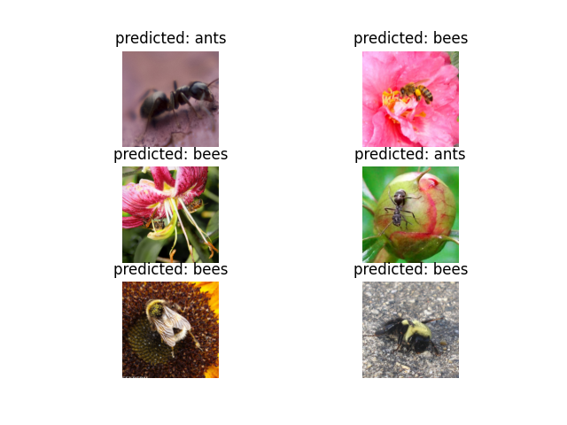
visualize_model(model_ft)

ConvNet as fixed feature extractor

Here, we need to freeze all the network except the final layer. We need to set requires_grad = False to freeze the parameters so that the gradients are not computed in backward().

You can read more about this in the documentation here.

model_conv = torchvision.models.resnet18(weights='IMAGENET1K_V1')
for param in model_conv.parameters():
    param.requires_grad = False

# Parameters of newly constructed modules have requires_grad=True by default
num_ftrs = model_conv.fc.in_features
model_conv.fc = nn.Linear(num_ftrs, 2)

model_conv = model_conv.to(device)

criterion = nn.CrossEntropyLoss()

# Observe that only parameters of final layer are being optimized as
# opposed to before.
optimizer_conv = optim.SGD(model_conv.fc.parameters(), lr=0.001, momentum=0.9)

# Decay LR by a factor of 0.1 every 7 epochs
exp_lr_scheduler = lr_scheduler.StepLR(optimizer_conv, step_size=7, gamma=0.1)

Train and evaluate

On CPU this will take about half the time compared to previous scenario. This is expected as gradients don’t need to be computed for most of the network. However, forward does need to be computed.

model_conv = train_model(model_conv, criterion, optimizer_conv,
                         exp_lr_scheduler, num_epochs=25)

Epoch 0/24
----------
train Loss: 0.6544 Acc: 0.6557
val Loss: 0.2520 Acc: 0.9150

Epoch 1/24
----------
train Loss: 0.4763 Acc: 0.7951
val Loss: 0.2074 Acc: 0.9216

Epoch 2/24
----------
train Loss: 0.4208 Acc: 0.7992
val Loss: 0.1770 Acc: 0.9542

Epoch 3/24
----------
train Loss: 0.4845 Acc: 0.7623
val Loss: 0.2678 Acc: 0.9020

Epoch 4/24
----------
train Loss: 0.4162 Acc: 0.7951
val Loss: 0.2538 Acc: 0.9150

Epoch 5/24
----------
train Loss: 0.5192 Acc: 0.7705
val Loss: 0.2392 Acc: 0.9085

Epoch 6/24
----------
train Loss: 0.4117 Acc: 0.8525
val Loss: 0.1615 Acc: 0.9542

Epoch 7/24
----------
train Loss: 0.3583 Acc: 0.8607
val Loss: 0.1855 Acc: 0.9477

Epoch 8/24
----------
train Loss: 0.4176 Acc: 0.8115
val Loss: 0.1699 Acc: 0.9542

Epoch 9/24
----------
train Loss: 0.2816 Acc: 0.8689
val Loss: 0.1909 Acc: 0.9281

Epoch 10/24
----------
train Loss: 0.3081 Acc: 0.8607
val Loss: 0.1935 Acc: 0.9281

Epoch 11/24
----------
train Loss: 0.3829 Acc: 0.8525
val Loss: 0.1710 Acc: 0.9542

Epoch 12/24
----------
train Loss: 0.3263 Acc: 0.8566
val Loss: 0.1677 Acc: 0.9542

Epoch 13/24
----------
train Loss: 0.3911 Acc: 0.8279
val Loss: 0.1682 Acc: 0.9542

Epoch 14/24
----------
train Loss: 0.3212 Acc: 0.8689
val Loss: 0.1723 Acc: 0.9542

Epoch 15/24
----------
train Loss: 0.3034 Acc: 0.8566
val Loss: 0.1745 Acc: 0.9346

Epoch 16/24
----------
train Loss: 0.3480 Acc: 0.8279
val Loss: 0.1722 Acc: 0.9608

Epoch 17/24
----------
train Loss: 0.2989 Acc: 0.8648
val Loss: 0.1650 Acc: 0.9542

Epoch 18/24
----------
train Loss: 0.2682 Acc: 0.8770
val Loss: 0.1880 Acc: 0.9346

Epoch 19/24
----------
train Loss: 0.3798 Acc: 0.8320
val Loss: 0.2156 Acc: 0.9216

Epoch 20/24
----------
train Loss: 0.2916 Acc: 0.8893
val Loss: 0.1735 Acc: 0.9542

Epoch 21/24
----------
train Loss: 0.2923 Acc: 0.8811
val Loss: 0.1710 Acc: 0.9477

Epoch 22/24
----------
train Loss: 0.3259 Acc: 0.8525
val Loss: 0.1645 Acc: 0.9542

Epoch 23/24
----------
train Loss: 0.3721 Acc: 0.8279
val Loss: 0.2199 Acc: 0.9216

Epoch 24/24
----------
train Loss: 0.3906 Acc: 0.8238
val Loss: 0.1794 Acc: 0.9477

Training complete in 0m 27s
Best val Acc: 0.960784

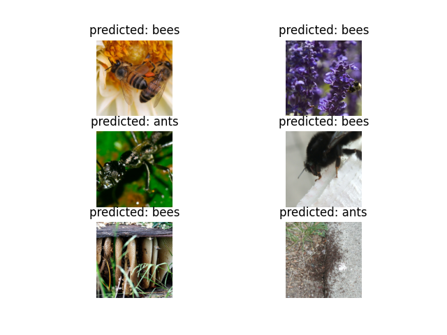
visualize_model(model_conv)

plt.ioff()
plt.show()

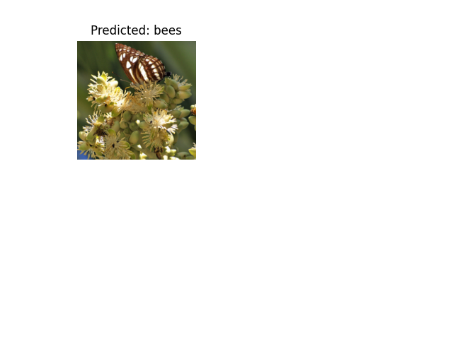
Inference on custom images

Use the trained model to make predictions on custom images and visualize the predicted class labels along with the images.

def visualize_model_predictions(model,img_path):
    was_training = model.training
    model.eval()

    img = Image.open(img_path)
    img = data_transforms['val'](img)
    img = img.unsqueeze(0)
    img = img.to(device)

    with torch.no_grad():
        outputs = model(img)
        _, preds = torch.max(outputs, 1)

        ax = plt.subplot(2,2,1)
        ax.axis('off')
        ax.set_title(f'Predicted: {class_names[preds[0]]}')
        imshow(img.cpu().data[0])

        model.train(mode=was_training)

visualize_model_predictions(
    model_conv,
    img_path='data/hymenoptera_data/val/bees/72100438_73de9f17af.jpg'
)

plt.ioff()
plt.show()

Further Learning

If you would like to learn more about the applications of transfer learning, checkout our Quantized Transfer Learning for Computer Vision Tutorial.