


Note
Go to the end to download the full example code.
Spatial Transformer Networks Tutorial#
Created On: Nov 08, 2017 | Last Updated: Jan 19, 2024 | Last Verified: Nov 05, 2024
Author: Ghassen HAMROUNI
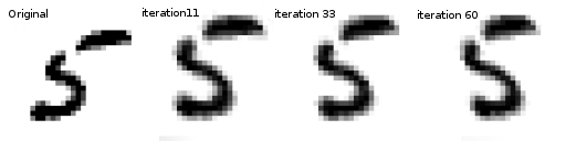
In this tutorial, you will learn how to augment your network using a visual attention mechanism called spatial transformer networks. You can read more about the spatial transformer networks in the DeepMind paper
Spatial transformer networks are a generalization of differentiable attention to any spatial transformation. Spatial transformer networks (STN for short) allow a neural network to learn how to perform spatial transformations on the input image in order to enhance the geometric invariance of the model. For example, it can crop a region of interest, scale and correct the orientation of an image. It can be a useful mechanism because CNNs are not invariant to rotation and scale and more general affine transformations.
One of the best things about STN is the ability to simply plug it into any existing CNN with very little modification.
# License: BSD
# Author: Ghassen Hamrouni

import torch
import torch.nn as nn
import torch.nn.functional as F
import torch.optim as optim
import torchvision
from torchvision import datasets, transforms
import matplotlib.pyplot as plt
import numpy as np

plt.ion()   # interactive mode
<contextlib.ExitStack object at 0x7f669ee2ae00>
Loading the data#
In this post we experiment with the classic MNIST dataset. Using a standard convolutional network augmented with a spatial transformer network.
from six.moves import urllib
opener = urllib.request.build_opener()
opener.addheaders = [('User-agent', 'Mozilla/5.0')]
urllib.request.install_opener(opener)

device = torch.device("cuda" if torch.cuda.is_available() else "cpu")

# Training dataset
train_loader = torch.utils.data.DataLoader(
    datasets.MNIST(root='.', train=True, download=True,
                   transform=transforms.Compose([
                       transforms.ToTensor(),
                       transforms.Normalize((0.1307,), (0.3081,))
                   ])), batch_size=64, shuffle=True, num_workers=4)
# Test dataset
test_loader = torch.utils.data.DataLoader(
    datasets.MNIST(root='.', train=False, transform=transforms.Compose([
        transforms.ToTensor(),
        transforms.Normalize((0.1307,), (0.3081,))
    ])), batch_size=64, shuffle=True, num_workers=4)
  0%|          | 0.00/9.91M [00:00<?, ?B/s]
100%|██████████| 9.91M/9.91M [00:00<00:00, 138MB/s]

  0%|          | 0.00/28.9k [00:00<?, ?B/s]
100%|██████████| 28.9k/28.9k [00:00<00:00, 31.0MB/s]

  0%|          | 0.00/1.65M [00:00<?, ?B/s]
100%|██████████| 1.65M/1.65M [00:00<00:00, 154MB/s]

  0%|          | 0.00/4.54k [00:00<?, ?B/s]
100%|██████████| 4.54k/4.54k [00:00<00:00, 24.5MB/s]
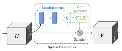
Depicting spatial transformer networks#
Spatial transformer networks boils down to three main components :
The localization network is a regular CNN which regresses the transformation parameters. The transformation is never learned explicitly from this dataset, instead the network learns automatically the spatial transformations that enhances the global accuracy.
The grid generator generates a grid of coordinates in the input image corresponding to each pixel from the output image.
The sampler uses the parameters of the transformation and applies it to the input image.
Note
We need the latest version of PyTorch that contains affine_grid and grid_sample modules.
class Net(nn.Module):
    def __init__(self):
        super(Net, self).__init__()
        self.conv1 = nn.Conv2d(1, 10, kernel_size=5)
        self.conv2 = nn.Conv2d(10, 20, kernel_size=5)
        self.conv2_drop = nn.Dropout2d()
        self.fc1 = nn.Linear(320, 50)
        self.fc2 = nn.Linear(50, 10)

        # Spatial transformer localization-network
        self.localization = nn.Sequential(
            nn.Conv2d(1, 8, kernel_size=7),
            nn.MaxPool2d(2, stride=2),
            nn.ReLU(True),
            nn.Conv2d(8, 10, kernel_size=5),
            nn.MaxPool2d(2, stride=2),
            nn.ReLU(True)
        )

        # Regressor for the 3 * 2 affine matrix
        self.fc_loc = nn.Sequential(
            nn.Linear(10 * 3 * 3, 32),
            nn.ReLU(True),
            nn.Linear(32, 3 * 2)
        )

        # Initialize the weights/bias with identity transformation
        self.fc_loc[2].weight.data.zero_()
        self.fc_loc[2].bias.data.copy_(torch.tensor([1, 0, 0, 0, 1, 0], dtype=torch.float))

    # Spatial transformer network forward function
    def stn(self, x):
        xs = self.localization(x)
        xs = xs.view(-1, 10 * 3 * 3)
        theta = self.fc_loc(xs)
        theta = theta.view(-1, 2, 3)

        grid = F.affine_grid(theta, x.size())
        x = F.grid_sample(x, grid)

        return x

    def forward(self, x):
        # transform the input
        x = self.stn(x)

        # Perform the usual forward pass
        x = F.relu(F.max_pool2d(self.conv1(x), 2))
        x = F.relu(F.max_pool2d(self.conv2_drop(self.conv2(x)), 2))
        x = x.view(-1, 320)
        x = F.relu(self.fc1(x))
        x = F.dropout(x, training=self.training)
        x = self.fc2(x)
        return F.log_softmax(x, dim=1)


model = Net().to(device)
Training the model#
Now, let’s use the SGD algorithm to train the model. The network is learning the classification task in a supervised way. In the same time the model is learning STN automatically in an end-to-end fashion.
optimizer = optim.SGD(model.parameters(), lr=0.01)


def train(epoch):
    model.train()
    for batch_idx, (data, target) in enumerate(train_loader):
        data, target = data.to(device), target.to(device)

        optimizer.zero_grad()
        output = model(data)
        loss = F.nll_loss(output, target)
        loss.backward()
        optimizer.step()
        if batch_idx % 500 == 0:
            print('Train Epoch: {} [{}/{} ({:.0f}%)]\tLoss: {:.6f}'.format(
                epoch, batch_idx * len(data), len(train_loader.dataset),
                100. * batch_idx / len(train_loader), loss.item()))
#
# A simple test procedure to measure the STN performances on MNIST.
#


def test():
    with torch.no_grad():
        model.eval()
        test_loss = 0
        correct = 0
        for data, target in test_loader:
            data, target = data.to(device), target.to(device)
            output = model(data)

            # sum up batch loss
            test_loss += F.nll_loss(output, target, size_average=False).item()
            # get the index of the max log-probability
            pred = output.max(1, keepdim=True)[1]
            correct += pred.eq(target.view_as(pred)).sum().item()

        test_loss /= len(test_loader.dataset)
        print('\nTest set: Average loss: {:.4f}, Accuracy: {}/{} ({:.0f}%)\n'
              .format(test_loss, correct, len(test_loader.dataset),
                      100. * correct / len(test_loader.dataset)))
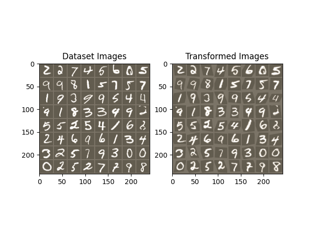
Visualizing the STN results#
Now, we will inspect the results of our learned visual attention mechanism.
We define a small helper function in order to visualize the transformations while training.
def convert_image_np(inp):
    """Convert a Tensor to numpy image."""
    inp = inp.numpy().transpose((1, 2, 0))
    mean = np.array([0.485, 0.456, 0.406])
    std = np.array([0.229, 0.224, 0.225])
    inp = std * inp + mean
    inp = np.clip(inp, 0, 1)
    return inp

# We want to visualize the output of the spatial transformers layer
# after the training, we visualize a batch of input images and
# the corresponding transformed batch using STN.


def visualize_stn():
    with torch.no_grad():
        # Get a batch of training data
        data = next(iter(test_loader))[0].to(device)

        input_tensor = data.cpu()
        transformed_input_tensor = model.stn(data).cpu()

        in_grid = convert_image_np(
            torchvision.utils.make_grid(input_tensor))

        out_grid = convert_image_np(
            torchvision.utils.make_grid(transformed_input_tensor))

        # Plot the results side-by-side
        f, axarr = plt.subplots(1, 2)
        axarr[0].imshow(in_grid)
        axarr[0].set_title('Dataset Images')

        axarr[1].imshow(out_grid)
        axarr[1].set_title('Transformed Images')

for epoch in range(1, 20 + 1):
    train(epoch)
    test()

# Visualize the STN transformation on some input batch
visualize_stn()

plt.ioff()
plt.show()
/var/lib/workspace/intermediate_source/spatial_transformer_tutorial.py:130: UserWarning: Default grid_sample and affine_grid behavior has changed to align_corners=False since 1.3.0. Please specify align_corners=True if the old behavior is desired. See the documentation of grid_sample for details.
  grid = F.affine_grid(theta, x.size())
/var/lib/workspace/intermediate_source/spatial_transformer_tutorial.py:131: UserWarning: Default grid_sample and affine_grid behavior has changed to align_corners=False since 1.3.0. Please specify align_corners=True if the old behavior is desired. See the documentation of grid_sample for details.
  x = F.grid_sample(x, grid)
Train Epoch: 1 [0/60000 (0%)]   Loss: 2.301495
Train Epoch: 1 [32000/60000 (53%)]      Loss: 0.590352
/var/lib/ci-user/.local/lib/python3.10/site-packages/torch/nn/functional.py:3230: UserWarning: size_average and reduce args will be deprecated, please use reduction='sum' instead.
  reduction = _Reduction.legacy_get_string(size_average, reduce)

Test set: Average loss: 0.2445, Accuracy: 9273/10000 (93%)

Train Epoch: 2 [0/60000 (0%)]   Loss: 0.588184
Train Epoch: 2 [32000/60000 (53%)]      Loss: 0.443036

Test set: Average loss: 0.1140, Accuracy: 9644/10000 (96%)

Train Epoch: 3 [0/60000 (0%)]   Loss: 0.104817
Train Epoch: 3 [32000/60000 (53%)]      Loss: 0.187283

Test set: Average loss: 0.2013, Accuracy: 9362/10000 (94%)

Train Epoch: 4 [0/60000 (0%)]   Loss: 0.467825
Train Epoch: 4 [32000/60000 (53%)]      Loss: 0.388502

Test set: Average loss: 0.0769, Accuracy: 9769/10000 (98%)

Train Epoch: 5 [0/60000 (0%)]   Loss: 0.214439
Train Epoch: 5 [32000/60000 (53%)]      Loss: 0.152647

Test set: Average loss: 0.0664, Accuracy: 9799/10000 (98%)

Train Epoch: 6 [0/60000 (0%)]   Loss: 0.133404
Train Epoch: 6 [32000/60000 (53%)]      Loss: 0.143182

Test set: Average loss: 0.0602, Accuracy: 9806/10000 (98%)

Train Epoch: 7 [0/60000 (0%)]   Loss: 0.121023
Train Epoch: 7 [32000/60000 (53%)]      Loss: 0.168223

Test set: Average loss: 0.0573, Accuracy: 9830/10000 (98%)

Train Epoch: 8 [0/60000 (0%)]   Loss: 0.065803
Train Epoch: 8 [32000/60000 (53%)]      Loss: 0.229770

Test set: Average loss: 0.0626, Accuracy: 9805/10000 (98%)

Train Epoch: 9 [0/60000 (0%)]   Loss: 0.096761
Train Epoch: 9 [32000/60000 (53%)]      Loss: 0.179188

Test set: Average loss: 0.0476, Accuracy: 9849/10000 (98%)

Train Epoch: 10 [0/60000 (0%)]  Loss: 0.040271
Train Epoch: 10 [32000/60000 (53%)]     Loss: 0.055136

Test set: Average loss: 0.0516, Accuracy: 9844/10000 (98%)

Train Epoch: 11 [0/60000 (0%)]  Loss: 0.035588
Train Epoch: 11 [32000/60000 (53%)]     Loss: 0.055403

Test set: Average loss: 0.0579, Accuracy: 9830/10000 (98%)

Train Epoch: 12 [0/60000 (0%)]  Loss: 0.275128
Train Epoch: 12 [32000/60000 (53%)]     Loss: 0.063360

Test set: Average loss: 0.0439, Accuracy: 9861/10000 (99%)

Train Epoch: 13 [0/60000 (0%)]  Loss: 0.184760
Train Epoch: 13 [32000/60000 (53%)]     Loss: 0.125527

Test set: Average loss: 0.0585, Accuracy: 9816/10000 (98%)

Train Epoch: 14 [0/60000 (0%)]  Loss: 0.105551
Train Epoch: 14 [32000/60000 (53%)]     Loss: 0.088872

Test set: Average loss: 0.0789, Accuracy: 9778/10000 (98%)

Train Epoch: 15 [0/60000 (0%)]  Loss: 0.103973
Train Epoch: 15 [32000/60000 (53%)]     Loss: 0.084506

Test set: Average loss: 0.0421, Accuracy: 9876/10000 (99%)

Train Epoch: 16 [0/60000 (0%)]  Loss: 0.222982
Train Epoch: 16 [32000/60000 (53%)]     Loss: 0.248119

Test set: Average loss: 0.0416, Accuracy: 9872/10000 (99%)

Train Epoch: 17 [0/60000 (0%)]  Loss: 0.202240
Train Epoch: 17 [32000/60000 (53%)]     Loss: 0.111763

Test set: Average loss: 0.3054, Accuracy: 9115/10000 (91%)

Train Epoch: 18 [0/60000 (0%)]  Loss: 0.482278
Train Epoch: 18 [32000/60000 (53%)]     Loss: 0.053312

Test set: Average loss: 0.0467, Accuracy: 9864/10000 (99%)

Train Epoch: 19 [0/60000 (0%)]  Loss: 0.061742
Train Epoch: 19 [32000/60000 (53%)]     Loss: 0.024329

Test set: Average loss: 0.0381, Accuracy: 9878/10000 (99%)

Train Epoch: 20 [0/60000 (0%)]  Loss: 0.188276
Train Epoch: 20 [32000/60000 (53%)]     Loss: 0.047986

Test set: Average loss: 0.0677, Accuracy: 9789/10000 (98%)
Total running time of the script: (1 minutes 37.355 seconds)