Audio Data Augmentation

Author: Moto Hira

torchaudio provides a variety of ways to augment audio data.

In this tutorial, we look into a way to apply effects, filters, RIR (room impulse response) and codecs.

At the end, we synthesize noisy speech over phone from clean speech.

import torch
import torchaudio
import torchaudio.functional as F

print(torch.__version__)
print(torchaudio.__version__)

import matplotlib.pyplot as plt

2.10.0.dev20251013+cu126
2.8.0a0+1d65bbe

Preparation

First, we import the modules and download the audio assets we use in this tutorial.

from IPython.display import Audio

from torchaudio.utils import _download_asset

SAMPLE_WAV = _download_asset("tutorial-assets/steam-train-whistle-daniel_simon.wav")
SAMPLE_RIR = _download_asset("tutorial-assets/Lab41-SRI-VOiCES-rm1-impulse-mc01-stu-clo-8000hz.wav")
SAMPLE_SPEECH = _download_asset("tutorial-assets/Lab41-SRI-VOiCES-src-sp0307-ch127535-sg0042-8000hz.wav")
SAMPLE_NOISE = _download_asset("tutorial-assets/Lab41-SRI-VOiCES-rm1-babb-mc01-stu-clo-8000hz.wav")

30.0%
59.9%
89.9%
100.0%

100.0%

100.0%

100.0%

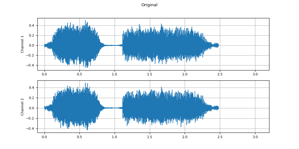
Loading the data

waveform1, sample_rate = torchaudio.load(SAMPLE_WAV, channels_first=False)

print(waveform1.shape, sample_rate)

torch.Size([109368, 2]) 44100

Let’s listen to the audio.

def plot_waveform(waveform, sample_rate, title="Waveform", xlim=None):
    waveform = waveform.numpy()

    num_channels, num_frames = waveform.shape
    time_axis = torch.arange(0, num_frames) / sample_rate

    figure, axes = plt.subplots(num_channels, 1)
    if num_channels == 1:
        axes = [axes]
    for c in range(num_channels):
        axes[c].plot(time_axis, waveform[c], linewidth=1)
        axes[c].grid(True)
        if num_channels > 1:
            axes[c].set_ylabel(f"Channel {c+1}")
        if xlim:
            axes[c].set_xlim(xlim)
    figure.suptitle(title)

def plot_specgram(waveform, sample_rate, title="Spectrogram", xlim=None):
    waveform = waveform.numpy()

    num_channels, _ = waveform.shape

    figure, axes = plt.subplots(num_channels, 1)
    if num_channels == 1:
        axes = [axes]
    for c in range(num_channels):
        axes[c].specgram(waveform[c], Fs=sample_rate)
        if num_channels > 1:
            axes[c].set_ylabel(f"Channel {c+1}")
        if xlim:
            axes[c].set_xlim(xlim)
    figure.suptitle(title)

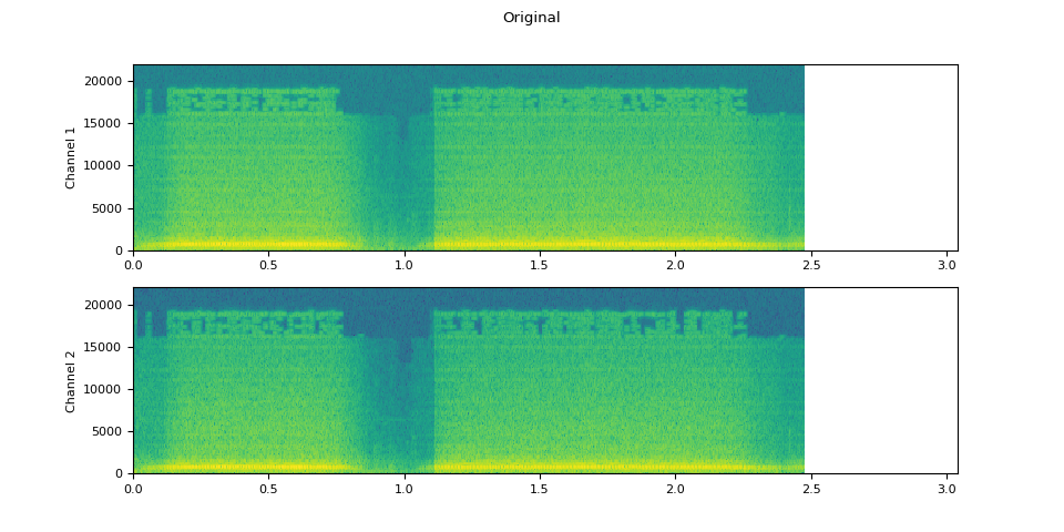
plot_waveform(waveform1.T, sample_rate, title="Original", xlim=(-0.1, 3.2))
plot_specgram(waveform1.T, sample_rate, title="Original", xlim=(0, 3.04))
Audio(waveform1.T, rate=sample_rate)

• 
• 

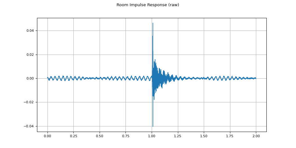
Simulating room reverberation

Convolution reverb is a technique that’s used to make clean audio sound as though it has been produced in a different environment.

Using Room Impulse Response (RIR), for instance, we can make clean speech sound as though it has been uttered in a conference room.

For this process, we need RIR data. The following data are from the VOiCES dataset, but you can record your own — just turn on your microphone and clap your hands.

rir_raw, sample_rate = torchaudio.load(SAMPLE_RIR)
plot_waveform(rir_raw, sample_rate, title="Room Impulse Response (raw)")
plot_specgram(rir_raw, sample_rate, title="Room Impulse Response (raw)")
Audio(rir_raw, rate=sample_rate)

• 
• 

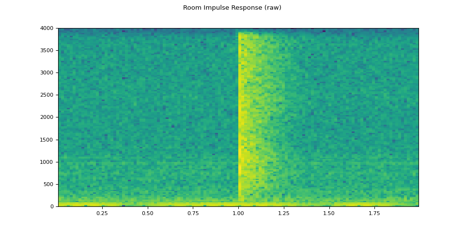
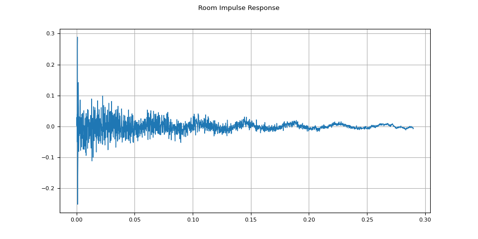
First, we need to clean up the RIR. We extract the main impulse and normalize it by its power.

rir = rir_raw[:, int(sample_rate * 1.01) : int(sample_rate * 1.3)]
rir = rir / torch.linalg.vector_norm(rir, ord=2)

plot_waveform(rir, sample_rate, title="Room Impulse Response")

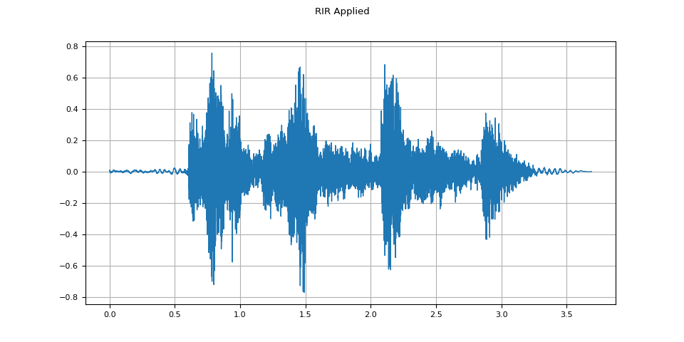
Then, using torchaudio.functional.fftconvolve(), we convolve the speech signal with the RIR.

speech, _ = torchaudio.load(SAMPLE_SPEECH)
augmented = F.fftconvolve(speech, rir)

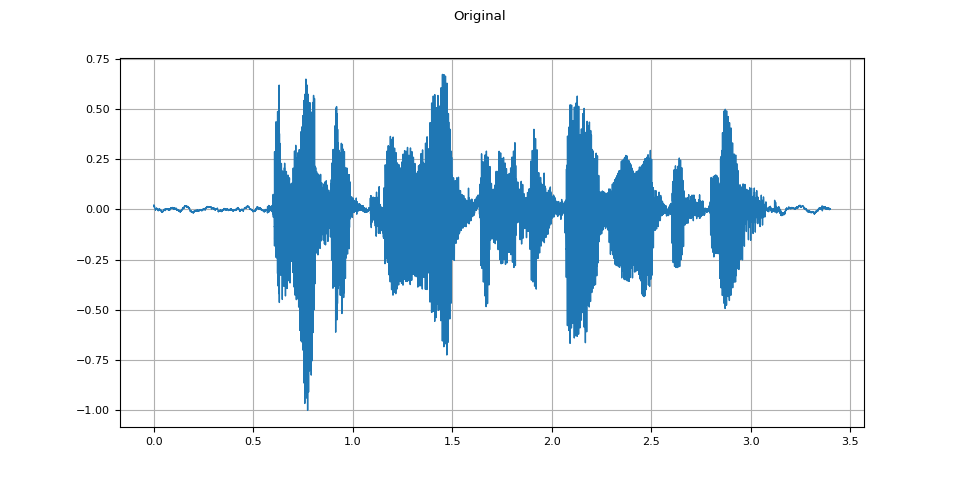
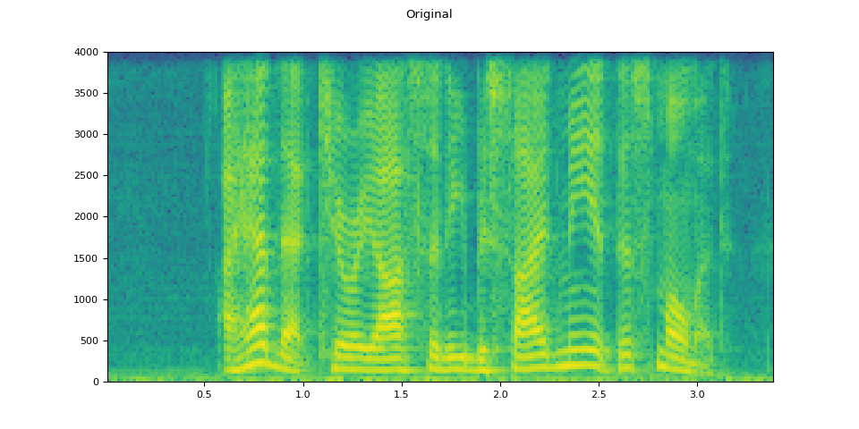
Original

plot_waveform(speech, sample_rate, title="Original")
plot_specgram(speech, sample_rate, title="Original")
Audio(speech, rate=sample_rate)

• 
• 

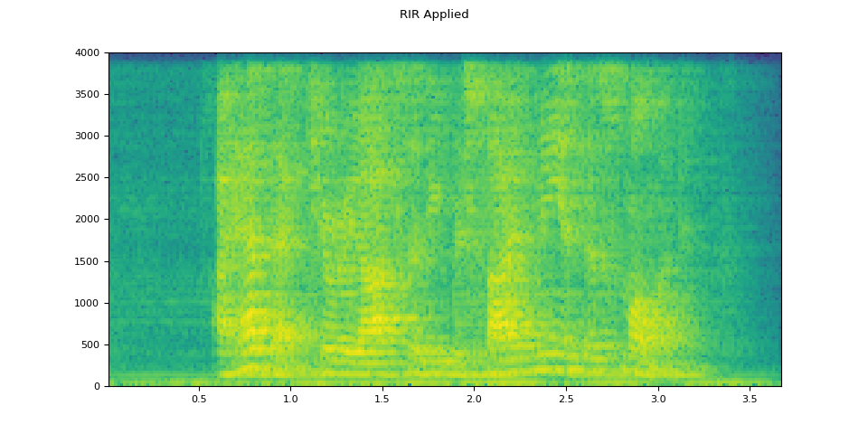
RIR applied

plot_waveform(augmented, sample_rate, title="RIR Applied")
plot_specgram(augmented, sample_rate, title="RIR Applied")
Audio(augmented, rate=sample_rate)

• 
• 

Adding background noise

To introduce background noise to audio data, we can add a noise Tensor to the Tensor representing the audio data according to some desired signal-to-noise ratio (SNR) [wikipedia], which determines the intensity of the audio data relative to that of the noise in the output.

$$ \mathrm{SNR} = \frac{P_{signal}}{P_{noise}} $$

$$ \mathrm{SNR_{dB}} = 10 \log _{{10}} \mathrm {SNR} $$

To add noise to audio data per SNRs, we use torchaudio.functional.add_noise().

speech, _ = torchaudio.load(SAMPLE_SPEECH)
noise, _ = torchaudio.load(SAMPLE_NOISE)
noise = noise[:, : speech.shape[1]]

snr_dbs = torch.tensor([20, 10, 3])
noisy_speeches = F.add_noise(speech, noise, snr_dbs)

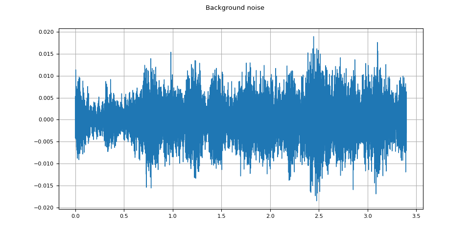
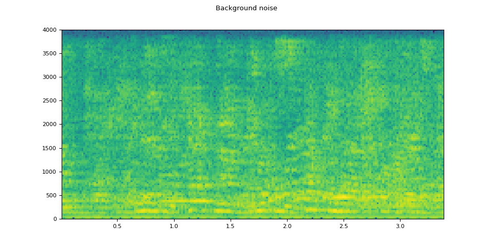
Background noise

plot_waveform(noise, sample_rate, title="Background noise")
plot_specgram(noise, sample_rate, title="Background noise")
Audio(noise, rate=sample_rate)

• 
• 

SNR 20 dB

snr_db, noisy_speech = snr_dbs[0], noisy_speeches[0:1]
plot_waveform(noisy_speech, sample_rate, title=f"SNR: {snr_db} [dB]")
plot_specgram(noisy_speech, sample_rate, title=f"SNR: {snr_db} [dB]")
Audio(noisy_speech, rate=sample_rate)

• 
• 

SNR 10 dB

snr_db, noisy_speech = snr_dbs[1], noisy_speeches[1:2]
plot_waveform(noisy_speech, sample_rate, title=f"SNR: {snr_db} [dB]")
plot_specgram(noisy_speech, sample_rate, title=f"SNR: {snr_db} [dB]")
Audio(noisy_speech, rate=sample_rate)

• 
• 

SNR 3 dB

snr_db, noisy_speech = snr_dbs[2], noisy_speeches[2:3]
plot_waveform(noisy_speech, sample_rate, title=f"SNR: {snr_db} [dB]")
plot_specgram(noisy_speech, sample_rate, title=f"SNR: {snr_db} [dB]")
Audio(noisy_speech, rate=sample_rate)

• 
•