torch.nn
Parameters
-
class
torch.nn.Parameter[source]¶ A kind of Tensor that is to be considered a module parameter.
Parameters are
Tensorsubclasses, that have a very special property when used withModules - when they’re assigned as Module attributes they are automatically added to the list of its parameters, and will appear e.g. inparameters()iterator. Assigning a Tensor doesn’t have such effect. This is because one might want to cache some temporary state, like last hidden state of the RNN, in the model. If there was no such class asParameter, these temporaries would get registered too.- Parameters
data (Tensor) – parameter tensor.
requires_grad (bool, optional) – if the parameter requires gradient. See Excluding subgraphs from backward for more details. Default: True
Containers
Module
-
class
torch.nn.Module[source]¶ Base class for all neural network modules.
Your models should also subclass this class.
Modules can also contain other Modules, allowing to nest them in a tree structure. You can assign the submodules as regular attributes:
import torch.nn as nn
import torch.nn.functional as F

class Model(nn.Module):
    def __init__(self):
        super(Model, self).__init__()
        self.conv1 = nn.Conv2d(1, 20, 5)
        self.conv2 = nn.Conv2d(20, 20, 5)

    def forward(self, x):
        x = F.relu(self.conv1(x))
        return F.relu(self.conv2(x))
Submodules assigned in this way will be registered, and will have their parameters converted too when you call
to(), etc.-
add_module(name, module)[source]¶ Adds a child module to the current module.
The module can be accessed as an attribute using the given name.
- Parameters
name (string) – name of the child module. The child module can be accessed from this module using the given name
module (Module) – child module to be added to the module.
-
apply(fn)[source]¶ Applies
fnrecursively to every submodule (as returned by.children()) as well as self. Typical use includes initializing the parameters of a model (see also torch.nn.init).- Parameters
fn (
Module-> None) – function to be applied to each submodule- Returns
self
- Return type
Example:
>>> @torch.no_grad()
>>> def init_weights(m):
>>>     print(m)
>>>     if type(m) == nn.Linear:
>>>         m.weight.fill_(1.0)
>>>         print(m.weight)
>>> net = nn.Sequential(nn.Linear(2, 2), nn.Linear(2, 2))
>>> net.apply(init_weights)
Linear(in_features=2, out_features=2, bias=True)
Parameter containing:
tensor([[ 1.,  1.],
        [ 1.,  1.]])
Linear(in_features=2, out_features=2, bias=True)
Parameter containing:
tensor([[ 1.,  1.],
        [ 1.,  1.]])
Sequential(
  (0): Linear(in_features=2, out_features=2, bias=True)
  (1): Linear(in_features=2, out_features=2, bias=True)
)
Sequential(
  (0): Linear(in_features=2, out_features=2, bias=True)
  (1): Linear(in_features=2, out_features=2, bias=True)
)
-
bfloat16()[source]¶ Casts all floating point parameters and buffers to
bfloat16datatype.- Returns
self
- Return type
-
buffers(recurse=True)[source]¶ Returns an iterator over module buffers.
- Parameters
recurse (bool) – if True, then yields buffers of this module and all submodules. Otherwise, yields only buffers that are direct members of this module.
- Yields
torch.Tensor – module buffer
Example:
>>> for buf in model.buffers():
>>>     print(type(buf), buf.size())
<class 'torch.Tensor'> (20L,)
<class 'torch.Tensor'> (20L, 1L, 5L, 5L)
-
children()[source]¶ Returns an iterator over immediate children modules.
- Yields
Module – a child module
-
cuda(device=None)[source]¶ Moves all model parameters and buffers to the GPU.
This also makes associated parameters and buffers different objects. So it should be called before constructing optimizer if the module will live on GPU while being optimized.
-
double()[source]¶ Casts all floating point parameters and buffers to
doubledatatype.- Returns
self
- Return type
-
dump_patches= False¶ This allows better BC support for
load_state_dict(). Instate_dict(), the version number will be saved as in the attribute _metadata of the returned state dict, and thus pickled. _metadata is a dictionary with keys that follow the naming convention of state dict. See_load_from_state_dicton how to use this information in loading.If new parameters/buffers are added/removed from a module, this number shall be bumped, and the module’s _load_from_state_dict method can compare the version number and do appropriate changes if the state dict is from before the change.
-
eval()[source]¶ Sets the module in evaluation mode.
This has any effect only on certain modules. See documentations of particular modules for details of their behaviors in training/evaluation mode, if they are affected, e.g.
Dropout,BatchNorm, etc.This is equivalent with
self.train(False).- Returns
self
- Return type
-
extra_repr()[source]¶ Set the extra representation of the module
To print customized extra information, you should reimplement this method in your own modules. Both single-line and multi-line strings are acceptable.
-
float()[source]¶ Casts all floating point parameters and buffers to float datatype.
- Returns
self
- Return type
-
forward(*input)[source]¶ Defines the computation performed at every call.
Should be overridden by all subclasses.
Note
Although the recipe for forward pass needs to be defined within this function, one should call the
Moduleinstance afterwards instead of this since the former takes care of running the registered hooks while the latter silently ignores them.
-
half()[source]¶ Casts all floating point parameters and buffers to
halfdatatype.- Returns
self
- Return type
-
load_state_dict(state_dict, strict=True)[source]¶ Copies parameters and buffers from
state_dictinto this module and its descendants. IfstrictisTrue, then the keys ofstate_dictmust exactly match the keys returned by this module’sstate_dict()function.- Parameters
state_dict (dict) – a dict containing parameters and persistent buffers.
strict (bool, optional) – whether to strictly enforce that the keys in
state_dictmatch the keys returned by this module’sstate_dict()function. Default:True
- Returns
missing_keys is a list of str containing the missing keys
unexpected_keys is a list of str containing the unexpected keys
- Return type
NamedTuplewithmissing_keysandunexpected_keysfields
-
modules()[source]¶ Returns an iterator over all modules in the network.
- Yields
Module – a module in the network
Note
Duplicate modules are returned only once. In the following example,
lwill be returned only once.Example:
>>> l = nn.Linear(2, 2)
>>> net = nn.Sequential(l, l)
>>> for idx, m in enumerate(net.modules()):
        print(idx, '->', m)

0 -> Sequential(
  (0): Linear(in_features=2, out_features=2, bias=True)
  (1): Linear(in_features=2, out_features=2, bias=True)
)
1 -> Linear(in_features=2, out_features=2, bias=True)
-
named_buffers(prefix='', recurse=True)[source]¶ Returns an iterator over module buffers, yielding both the name of the buffer as well as the buffer itself.
- Parameters
- Yields
(string, torch.Tensor) – Tuple containing the name and buffer
Example:
>>> for name, buf in self.named_buffers():
>>>    if name in ['running_var']:
>>>        print(buf.size())
-
named_children()[source]¶ Returns an iterator over immediate children modules, yielding both the name of the module as well as the module itself.
- Yields
(string, Module) – Tuple containing a name and child module
Example:
>>> for name, module in model.named_children():
>>>     if name in ['conv4', 'conv5']:
>>>         print(module)
-
named_modules(memo=None, prefix='')[source]¶ Returns an iterator over all modules in the network, yielding both the name of the module as well as the module itself.
- Yields
(string, Module) – Tuple of name and module
Note
Duplicate modules are returned only once. In the following example,
lwill be returned only once.Example:
>>> l = nn.Linear(2, 2)
>>> net = nn.Sequential(l, l)
>>> for idx, m in enumerate(net.named_modules()):
        print(idx, '->', m)

0 -> ('', Sequential(
  (0): Linear(in_features=2, out_features=2, bias=True)
  (1): Linear(in_features=2, out_features=2, bias=True)
))
1 -> ('0', Linear(in_features=2, out_features=2, bias=True))
-
named_parameters(prefix='', recurse=True)[source]¶ Returns an iterator over module parameters, yielding both the name of the parameter as well as the parameter itself.
- Parameters
- Yields
(string, Parameter) – Tuple containing the name and parameter
Example:
>>> for name, param in self.named_parameters():
>>>    if name in ['bias']:
>>>        print(param.size())
-
parameters(recurse=True)[source]¶ Returns an iterator over module parameters.
This is typically passed to an optimizer.
- Parameters
recurse (bool) – if True, then yields parameters of this module and all submodules. Otherwise, yields only parameters that are direct members of this module.
- Yields
Parameter – module parameter
Example:
>>> for param in model.parameters():
>>>     print(type(param), param.size())
<class 'torch.Tensor'> (20L,)
<class 'torch.Tensor'> (20L, 1L, 5L, 5L)
-
register_backward_hook(hook)[source]¶ Registers a backward hook on the module.
The hook will be called every time the gradients with respect to module inputs are computed. The hook should have the following signature:
hook(module, grad_input, grad_output) -> Tensor or None
The
grad_inputandgrad_outputmay be tuples if the module has multiple inputs or outputs. The hook should not modify its arguments, but it can optionally return a new gradient with respect to input that will be used in place ofgrad_inputin subsequent computations.- Returns
a handle that can be used to remove the added hook by calling
handle.remove()- Return type
torch.utils.hooks.RemovableHandle
Warning
The current implementation will not have the presented behavior for complex
Modulethat perform many operations. In some failure cases,grad_inputandgrad_outputwill only contain the gradients for a subset of the inputs and outputs. For suchModule, you should usetorch.Tensor.register_hook()directly on a specific input or output to get the required gradients.
-
register_buffer(name, tensor)[source]¶ Adds a persistent buffer to the module.
This is typically used to register a buffer that should not to be considered a model parameter. For example, BatchNorm’s
running_meanis not a parameter, but is part of the persistent state.Buffers can be accessed as attributes using given names.
- Parameters
name (string) – name of the buffer. The buffer can be accessed from this module using the given name
tensor (Tensor) – buffer to be registered.
Example:
>>> self.register_buffer('running_mean', torch.zeros(num_features))
-
register_forward_hook(hook)[source]¶ Registers a forward hook on the module.
The hook will be called every time after
forward()has computed an output. It should have the following signature:hook(module, input, output) -> None or modified output
The hook can modify the output. It can modify the input inplace but it will not have effect on forward since this is called after
forward()is called.- Returns
a handle that can be used to remove the added hook by calling
handle.remove()- Return type
torch.utils.hooks.RemovableHandle
-
register_forward_pre_hook(hook)[source]¶ Registers a forward pre-hook on the module.
The hook will be called every time before
forward()is invoked. It should have the following signature:hook(module, input) -> None or modified input
The hook can modify the input. User can either return a tuple or a single modified value in the hook. We will wrap the value into a tuple if a single value is returned(unless that value is already a tuple).
- Returns
a handle that can be used to remove the added hook by calling
handle.remove()- Return type
torch.utils.hooks.RemovableHandle
-
register_parameter(name, param)[source]¶ Adds a parameter to the module.
The parameter can be accessed as an attribute using given name.
- Parameters
name (string) – name of the parameter. The parameter can be accessed from this module using the given name
param (Parameter) – parameter to be added to the module.
-
requires_grad_(requires_grad=True)[source]¶ Change if autograd should record operations on parameters in this module.
This method sets the parameters’
requires_gradattributes in-place.This method is helpful for freezing part of the module for finetuning or training parts of a model individually (e.g., GAN training).
-
state_dict(destination=None, prefix='', keep_vars=False)[source]¶ Returns a dictionary containing a whole state of the module.
Both parameters and persistent buffers (e.g. running averages) are included. Keys are corresponding parameter and buffer names.
- Returns
a dictionary containing a whole state of the module
- Return type
Example:
>>> module.state_dict().keys()
['bias', 'weight']
-
to(*args, **kwargs)[source]¶ Moves and/or casts the parameters and buffers.
This can be called as
-
to(device=None, dtype=None, non_blocking=False)[source]
-
to(dtype, non_blocking=False)[source]
-
to(tensor, non_blocking=False)[source]
-
to(memory_format=torch.channels_last)[source]
Its signature is similar to
torch.Tensor.to(), but only accepts floating point desireddtypes. In addition, this method will only cast the floating point parameters and buffers todtype(if given). The integral parameters and buffers will be moveddevice, if that is given, but with dtypes unchanged. Whennon_blockingis set, it tries to convert/move asynchronously with respect to the host if possible, e.g., moving CPU Tensors with pinned memory to CUDA devices.See below for examples.
Note
This method modifies the module in-place.
- Parameters
device (
torch.device) – the desired device of the parameters and buffers in this moduledtype (
torch.dtype) – the desired floating point type of the floating point parameters and buffers in this moduletensor (torch.Tensor) – Tensor whose dtype and device are the desired dtype and device for all parameters and buffers in this module
memory_format (
torch.memory_format) – the desired memory format for 4D parameters and buffers in this module (keyword only argument)
- Returns
self
- Return type
Example:
>>> linear = nn.Linear(2, 2)
>>> linear.weight
Parameter containing:
tensor([[ 0.1913, -0.3420],
        [-0.5113, -0.2325]])
>>> linear.to(torch.double)
Linear(in_features=2, out_features=2, bias=True)
>>> linear.weight
Parameter containing:
tensor([[ 0.1913, -0.3420],
        [-0.5113, -0.2325]], dtype=torch.float64)
>>> gpu1 = torch.device("cuda:1")
>>> linear.to(gpu1, dtype=torch.half, non_blocking=True)
Linear(in_features=2, out_features=2, bias=True)
>>> linear.weight
Parameter containing:
tensor([[ 0.1914, -0.3420],
        [-0.5112, -0.2324]], dtype=torch.float16, device='cuda:1')
>>> cpu = torch.device("cpu")
>>> linear.to(cpu)
Linear(in_features=2, out_features=2, bias=True)
>>> linear.weight
Parameter containing:
tensor([[ 0.1914, -0.3420],
        [-0.5112, -0.2324]], dtype=torch.float16)
-
-
train(mode=True)[source]¶ Sets the module in training mode.
This has any effect only on certain modules. See documentations of particular modules for details of their behaviors in training/evaluation mode, if they are affected, e.g.
Dropout,BatchNorm, etc.
-
Sequential
-
class
torch.nn.Sequential(*args)[source]¶ A sequential container. Modules will be added to it in the order they are passed in the constructor. Alternatively, an ordered dict of modules can also be passed in.
To make it easier to understand, here is a small example:
# Example of using Sequential
model = nn.Sequential(
          nn.Conv2d(1,20,5),
          nn.ReLU(),
          nn.Conv2d(20,64,5),
          nn.ReLU()
        )

# Example of using Sequential with OrderedDict
model = nn.Sequential(OrderedDict([
          ('conv1', nn.Conv2d(1,20,5)),
          ('relu1', nn.ReLU()),
          ('conv2', nn.Conv2d(20,64,5)),
          ('relu2', nn.ReLU())
        ]))
ModuleList
-
class
torch.nn.ModuleList(modules=None)[source]¶ Holds submodules in a list.
ModuleListcan be indexed like a regular Python list, but modules it contains are properly registered, and will be visible by allModulemethods.- Parameters
modules (iterable, optional) – an iterable of modules to add
Example:
class MyModule(nn.Module):
    def __init__(self):
        super(MyModule, self).__init__()
        self.linears = nn.ModuleList([nn.Linear(10, 10) for i in range(10)])

    def forward(self, x):
        # ModuleList can act as an iterable, or be indexed using ints
        for i, l in enumerate(self.linears):
            x = self.linears[i // 2](x) + l(x)
        return x
-
append(module)[source]¶ Appends a given module to the end of the list.
- Parameters
module (nn.Module) – module to append
ModuleDict
-
class
torch.nn.ModuleDict(modules=None)[source]¶ Holds submodules in a dictionary.
ModuleDictcan be indexed like a regular Python dictionary, but modules it contains are properly registered, and will be visible by allModulemethods.ModuleDictis an ordered dictionary that respectsthe order of insertion, and
in
update(), the order of the mergedOrderedDictor anotherModuleDict(the argument toupdate()).
Note that
update()with other unordered mapping types (e.g., Python’s plaindict) does not preserve the order of the merged mapping.- Parameters
modules (iterable, optional) – a mapping (dictionary) of (string: module) or an iterable of key-value pairs of type (string, module)
Example:
class MyModule(nn.Module):
    def __init__(self):
        super(MyModule, self).__init__()
        self.choices = nn.ModuleDict({
                'conv': nn.Conv2d(10, 10, 3),
                'pool': nn.MaxPool2d(3)
        })
        self.activations = nn.ModuleDict([
                ['lrelu', nn.LeakyReLU()],
                ['prelu', nn.PReLU()]
        ])

    def forward(self, x, choice, act):
        x = self.choices[choice](x)
        x = self.activations[act](x)
        return x
-
pop(key)[source]¶ Remove key from the ModuleDict and return its module.
- Parameters
key (string) – key to pop from the ModuleDict
-
update(modules)[source]¶ Update the
ModuleDictwith the key-value pairs from a mapping or an iterable, overwriting existing keys.Note
If
modulesis anOrderedDict, aModuleDict, or an iterable of key-value pairs, the order of new elements in it is preserved.
ParameterList
-
class
torch.nn.ParameterList(parameters=None)[source]¶ Holds parameters in a list.
ParameterListcan be indexed like a regular Python list, but parameters it contains are properly registered, and will be visible by allModulemethods.- Parameters
parameters (iterable, optional) – an iterable of
Parameterto add
Example:
class MyModule(nn.Module):
    def __init__(self):
        super(MyModule, self).__init__()
        self.params = nn.ParameterList([nn.Parameter(torch.randn(10, 10)) for i in range(10)])

    def forward(self, x):
        # ParameterList can act as an iterable, or be indexed using ints
        for i, p in enumerate(self.params):
            x = self.params[i // 2].mm(x) + p.mm(x)
        return x
-
append(parameter)[source]¶ Appends a given parameter at the end of the list.
- Parameters
parameter (nn.Parameter) – parameter to append
ParameterDict
-
class
torch.nn.ParameterDict(parameters=None)[source]¶ Holds parameters in a dictionary.
ParameterDict can be indexed like a regular Python dictionary, but parameters it contains are properly registered, and will be visible by all Module methods.
ParameterDictis an ordered dictionary that respectsthe order of insertion, and
in
update(), the order of the mergedOrderedDictor anotherParameterDict(the argument toupdate()).
Note that
update()with other unordered mapping types (e.g., Python’s plaindict) does not preserve the order of the merged mapping.- Parameters
parameters (iterable, optional) – a mapping (dictionary) of (string :
Parameter) or an iterable of key-value pairs of type (string,Parameter)
Example:
class MyModule(nn.Module):
    def __init__(self):
        super(MyModule, self).__init__()
        self.params = nn.ParameterDict({
                'left': nn.Parameter(torch.randn(5, 10)),
                'right': nn.Parameter(torch.randn(5, 10))
        })

    def forward(self, x, choice):
        x = self.params[choice].mm(x)
        return x
-
pop(key)[source]¶ Remove key from the ParameterDict and return its parameter.
- Parameters
key (string) – key to pop from the ParameterDict
-
update(parameters)[source]¶ Update the
ParameterDictwith the key-value pairs from a mapping or an iterable, overwriting existing keys.Note
If
parametersis anOrderedDict, aParameterDict, or an iterable of key-value pairs, the order of new elements in it is preserved.
Convolution layers
Conv1d
-
class
torch.nn.Conv1d(in_channels, out_channels, kernel_size, stride=1, padding=0, dilation=1, groups=1, bias=True, padding_mode='zeros')[source]¶ Applies a 1D convolution over an input signal composed of several input planes.
In the simplest case, the output value of the layer with input size and output can be precisely described as:
where is the valid cross-correlation operator, is a batch size, denotes a number of channels, is a length of signal sequence.
stridecontrols the stride for the cross-correlation, a single number or a one-element tuple.paddingcontrols the amount of implicit zero-paddings on both sides forpaddingnumber of points.dilationcontrols the spacing between the kernel points; also known as the à trous algorithm. It is harder to describe, but this link has a nice visualization of whatdilationdoes.groupscontrols the connections between inputs and outputs.in_channelsandout_channelsmust both be divisible bygroups. For example,At groups=1, all inputs are convolved to all outputs.
At groups=2, the operation becomes equivalent to having two conv layers side by side, each seeing half the input channels, and producing half the output channels, and both subsequently concatenated.
At groups=
in_channels, each input channel is convolved with its own set of filters, of size .
Note
Depending of the size of your kernel, several (of the last) columns of the input might be lost, because it is a valid cross-correlation, and not a full cross-correlation. It is up to the user to add proper padding.
Note
When groups == in_channels and out_channels == K * in_channels, where K is a positive integer, this operation is also termed in literature as depthwise convolution.
In other words, for an input of size , a depthwise convolution with a depthwise multiplier K, can be constructed by arguments .
Note
In some circumstances when using the CUDA backend with CuDNN, this operator may select a nondeterministic algorithm to increase performance. If this is undesirable, you can try to make the operation deterministic (potentially at a performance cost) by setting
torch.backends.cudnn.deterministic =
True
. Please see the notes on Reproducibility for background.- Parameters
in_channels (int) – Number of channels in the input image
out_channels (int) – Number of channels produced by the convolution
stride (int or tuple, optional) – Stride of the convolution. Default: 1
padding (int or tuple, optional) – Zero-padding added to both sides of the input. Default: 0
padding_mode (string, optional) –
'zeros','reflect','replicate'or'circular'. Default:'zeros'dilation (int or tuple, optional) – Spacing between kernel elements. Default: 1
groups (int, optional) – Number of blocked connections from input channels to output channels. Default: 1
bias (bool, optional) – If
True, adds a learnable bias to the output. Default:True
- Shape:
Input:
Output: where
- Variables
Examples:
>>> m = nn.Conv1d(16, 33, 3, stride=2)
>>> input = torch.randn(20, 16, 50)
>>> output = m(input)
Conv2d
-
class
torch.nn.Conv2d(in_channels, out_channels, kernel_size, stride=1, padding=0, dilation=1, groups=1, bias=True, padding_mode='zeros')[source]¶ Applies a 2D convolution over an input signal composed of several input planes.
In the simplest case, the output value of the layer with input size and output can be precisely described as:
where is the valid 2D cross-correlation operator, is a batch size, denotes a number of channels, is a height of input planes in pixels, and is width in pixels.
stridecontrols the stride for the cross-correlation, a single number or a tuple.paddingcontrols the amount of implicit zero-paddings on both sides forpaddingnumber of points for each dimension.dilationcontrols the spacing between the kernel points; also known as the à trous algorithm. It is harder to describe, but this link has a nice visualization of whatdilationdoes.groupscontrols the connections between inputs and outputs.in_channelsandout_channelsmust both be divisible bygroups. For example,At groups=1, all inputs are convolved to all outputs.
At groups=2, the operation becomes equivalent to having two conv layers side by side, each seeing half the input channels, and producing half the output channels, and both subsequently concatenated.
At groups=
in_channels, each input channel is convolved with its own set of filters, of size: .
The parameters
kernel_size,stride,padding,dilationcan either be:a single
int– in which case the same value is used for the height and width dimensiona
tupleof two ints – in which case, the first int is used for the height dimension, and the second int for the width dimension
Note
Depending of the size of your kernel, several (of the last) columns of the input might be lost, because it is a valid cross-correlation, and not a full cross-correlation. It is up to the user to add proper padding.
Note
When groups == in_channels and out_channels == K * in_channels, where K is a positive integer, this operation is also termed in literature as depthwise convolution.
In other words, for an input of size , a depthwise convolution with a depthwise multiplier K, can be constructed by arguments .
Note
In some circumstances when using the CUDA backend with CuDNN, this operator may select a nondeterministic algorithm to increase performance. If this is undesirable, you can try to make the operation deterministic (potentially at a performance cost) by setting
torch.backends.cudnn.deterministic =
True
. Please see the notes on Reproducibility for background.- Parameters
in_channels (int) – Number of channels in the input image
out_channels (int) – Number of channels produced by the convolution
stride (int or tuple, optional) – Stride of the convolution. Default: 1
padding (int or tuple, optional) – Zero-padding added to both sides of the input. Default: 0
padding_mode (string, optional) –
'zeros','reflect','replicate'or'circular'. Default:'zeros'dilation (int or tuple, optional) – Spacing between kernel elements. Default: 1
groups (int, optional) – Number of blocked connections from input channels to output channels. Default: 1
bias (bool, optional) – If
True, adds a learnable bias to the output. Default:True
- Shape:
Input:
Output: where
- Variables
Examples:
>>> # With square kernels and equal stride
>>> m = nn.Conv2d(16, 33, 3, stride=2)
>>> # non-square kernels and unequal stride and with padding
>>> m = nn.Conv2d(16, 33, (3, 5), stride=(2, 1), padding=(4, 2))
>>> # non-square kernels and unequal stride and with padding and dilation
>>> m = nn.Conv2d(16, 33, (3, 5), stride=(2, 1), padding=(4, 2), dilation=(3, 1))
>>> input = torch.randn(20, 16, 50, 100)
>>> output = m(input)
Conv3d
-
class
torch.nn.Conv3d(in_channels, out_channels, kernel_size, stride=1, padding=0, dilation=1, groups=1, bias=True, padding_mode='zeros')[source]¶ Applies a 3D convolution over an input signal composed of several input planes.
In the simplest case, the output value of the layer with input size and output can be precisely described as:
where is the valid 3D cross-correlation operator
stridecontrols the stride for the cross-correlation.paddingcontrols the amount of implicit zero-paddings on both sides forpaddingnumber of points for each dimension.dilationcontrols the spacing between the kernel points; also known as the à trous algorithm. It is harder to describe, but this link has a nice visualization of whatdilationdoes.groupscontrols the connections between inputs and outputs.in_channelsandout_channelsmust both be divisible bygroups. For example,At groups=1, all inputs are convolved to all outputs.
At groups=2, the operation becomes equivalent to having two conv layers side by side, each seeing half the input channels, and producing half the output channels, and both subsequently concatenated.
At groups=
in_channels, each input channel is convolved with its own set of filters, of size .
The parameters
kernel_size,stride,padding,dilationcan either be:a single
int– in which case the same value is used for the depth, height and width dimensiona
tupleof three ints – in which case, the first int is used for the depth dimension, the second int for the height dimension and the third int for the width dimension
Note
Depending of the size of your kernel, several (of the last) columns of the input might be lost, because it is a valid cross-correlation, and not a full cross-correlation. It is up to the user to add proper padding.
Note
When groups == in_channels and out_channels == K * in_channels, where K is a positive integer, this operation is also termed in literature as depthwise convolution.
In other words, for an input of size , a depthwise convolution with a depthwise multiplier K, can be constructed by arguments .
Note
In some circumstances when using the CUDA backend with CuDNN, this operator may select a nondeterministic algorithm to increase performance. If this is undesirable, you can try to make the operation deterministic (potentially at a performance cost) by setting
torch.backends.cudnn.deterministic =
True
. Please see the notes on Reproducibility for background.- Parameters
in_channels (int) – Number of channels in the input image
out_channels (int) – Number of channels produced by the convolution
stride (int or tuple, optional) – Stride of the convolution. Default: 1
padding (int or tuple, optional) – Zero-padding added to all three sides of the input. Default: 0
padding_mode (string, optional) –
'zeros','reflect','replicate'or'circular'. Default:'zeros'dilation (int or tuple, optional) – Spacing between kernel elements. Default: 1
groups (int, optional) – Number of blocked connections from input channels to output channels. Default: 1
bias (bool, optional) – If
True, adds a learnable bias to the output. Default:True
- Shape:
Input:
Output: where
- Variables
Examples:
>>> # With square kernels and equal stride
>>> m = nn.Conv3d(16, 33, 3, stride=2)
>>> # non-square kernels and unequal stride and with padding
>>> m = nn.Conv3d(16, 33, (3, 5, 2), stride=(2, 1, 1), padding=(4, 2, 0))
>>> input = torch.randn(20, 16, 10, 50, 100)
>>> output = m(input)
ConvTranspose1d
-
class
torch.nn.ConvTranspose1d(in_channels, out_channels, kernel_size, stride=1, padding=0, output_padding=0, groups=1, bias=True, dilation=1, padding_mode='zeros')[source]¶ Applies a 1D transposed convolution operator over an input image composed of several input planes.
This module can be seen as the gradient of Conv1d with respect to its input. It is also known as a fractionally-strided convolution or a deconvolution (although it is not an actual deconvolution operation).
stridecontrols the stride for the cross-correlation.paddingcontrols the amount of implicit zero-paddings on both sides fordilation * (kernel_size - 1) - paddingnumber of points. See note below for details.output_paddingcontrols the additional size added to one side of the output shape. See note below for details.dilationcontrols the spacing between the kernel points; also known as the à trous algorithm. It is harder to describe, but this link has a nice visualization of whatdilationdoes.groupscontrols the connections between inputs and outputs.in_channelsandout_channelsmust both be divisible bygroups. For example,At groups=1, all inputs are convolved to all outputs.
At groups=2, the operation becomes equivalent to having two conv layers side by side, each seeing half the input channels, and producing half the output channels, and both subsequently concatenated.
At groups=
in_channels, each input channel is convolved with its own set of filters (of size ).
Note
Depending of the size of your kernel, several (of the last) columns of the input might be lost, because it is a valid cross-correlation, and not a full cross-correlation. It is up to the user to add proper padding.
Note
The
paddingargument effectively addsdilation * (kernel_size - 1) - paddingamount of zero padding to both sizes of the input. This is set so that when aConv1dand aConvTranspose1dare initialized with same parameters, they are inverses of each other in regard to the input and output shapes. However, whenstride > 1,Conv1dmaps multiple input shapes to the same output shape.output_paddingis provided to resolve this ambiguity by effectively increasing the calculated output shape on one side. Note thatoutput_paddingis only used to find output shape, but does not actually add zero-padding to output.Note
In some circumstances when using the CUDA backend with CuDNN, this operator may select a nondeterministic algorithm to increase performance. If this is undesirable, you can try to make the operation deterministic (potentially at a performance cost) by setting
torch.backends.cudnn.deterministic =
True
. Please see the notes on Reproducibility for background.- Parameters
in_channels (int) – Number of channels in the input image
out_channels (int) – Number of channels produced by the convolution
stride (int or tuple, optional) – Stride of the convolution. Default: 1
padding (int or tuple, optional) –
dilation * (kernel_size - 1) - paddingzero-padding will be added to both sides of the input. Default: 0output_padding (int or tuple, optional) – Additional size added to one side of the output shape. Default: 0
groups (int, optional) – Number of blocked connections from input channels to output channels. Default: 1
bias (bool, optional) – If
True, adds a learnable bias to the output. Default:Truedilation (int or tuple, optional) – Spacing between kernel elements. Default: 1
- Shape:
Input:
Output: where
- Variables
ConvTranspose2d
-
class
torch.nn.ConvTranspose2d(in_channels, out_channels, kernel_size, stride=1, padding=0, output_padding=0, groups=1, bias=True, dilation=1, padding_mode='zeros')[source]¶ Applies a 2D transposed convolution operator over an input image composed of several input planes.
This module can be seen as the gradient of Conv2d with respect to its input. It is also known as a fractionally-strided convolution or a deconvolution (although it is not an actual deconvolution operation).
stridecontrols the stride for the cross-correlation.paddingcontrols the amount of implicit zero-paddings on both sides fordilation * (kernel_size - 1) - paddingnumber of points. See note below for details.output_paddingcontrols the additional size added to one side of the output shape. See note below for details.dilationcontrols the spacing between the kernel points; also known as the à trous algorithm. It is harder to describe, but this link has a nice visualization of whatdilationdoes.groupscontrols the connections between inputs and outputs.in_channelsandout_channelsmust both be divisible bygroups. For example,At groups=1, all inputs are convolved to all outputs.
At groups=2, the operation becomes equivalent to having two conv layers side by side, each seeing half the input channels, and producing half the output channels, and both subsequently concatenated.
At groups=
in_channels, each input channel is convolved with its own set of filters (of size ).
The parameters
kernel_size,stride,padding,output_paddingcan either be:a single
int– in which case the same value is used for the height and width dimensionsa
tupleof two ints – in which case, the first int is used for the height dimension, and the second int for the width dimension
Note
Depending of the size of your kernel, several (of the last) columns of the input might be lost, because it is a valid cross-correlation, and not a full cross-correlation. It is up to the user to add proper padding.
Note
The
paddingargument effectively addsdilation * (kernel_size - 1) - paddingamount of zero padding to both sizes of the input. This is set so that when aConv2dand aConvTranspose2dare initialized with same parameters, they are inverses of each other in regard to the input and output shapes. However, whenstride > 1,Conv2dmaps multiple input shapes to the same output shape.output_paddingis provided to resolve this ambiguity by effectively increasing the calculated output shape on one side. Note thatoutput_paddingis only used to find output shape, but does not actually add zero-padding to output.Note
In some circumstances when using the CUDA backend with CuDNN, this operator may select a nondeterministic algorithm to increase performance. If this is undesirable, you can try to make the operation deterministic (potentially at a performance cost) by setting
torch.backends.cudnn.deterministic =
True
. Please see the notes on Reproducibility for background.- Parameters
in_channels (int) – Number of channels in the input image
out_channels (int) – Number of channels produced by the convolution
stride (int or tuple, optional) – Stride of the convolution. Default: 1
padding (int or tuple, optional) –
dilation * (kernel_size - 1) - paddingzero-padding will be added to both sides of each dimension in the input. Default: 0output_padding (int or tuple, optional) – Additional size added to one side of each dimension in the output shape. Default: 0
groups (int, optional) – Number of blocked connections from input channels to output channels. Default: 1
bias (bool, optional) – If
True, adds a learnable bias to the output. Default:Truedilation (int or tuple, optional) – Spacing between kernel elements. Default: 1
- Shape:
Input:
Output: where
- Variables
Examples:
>>> # With square kernels and equal stride
>>> m = nn.ConvTranspose2d(16, 33, 3, stride=2)
>>> # non-square kernels and unequal stride and with padding
>>> m = nn.ConvTranspose2d(16, 33, (3, 5), stride=(2, 1), padding=(4, 2))
>>> input = torch.randn(20, 16, 50, 100)
>>> output = m(input)
>>> # exact output size can be also specified as an argument
>>> input = torch.randn(1, 16, 12, 12)
>>> downsample = nn.Conv2d(16, 16, 3, stride=2, padding=1)
>>> upsample = nn.ConvTranspose2d(16, 16, 3, stride=2, padding=1)
>>> h = downsample(input)
>>> h.size()
torch.Size([1, 16, 6, 6])
>>> output = upsample(h, output_size=input.size())
>>> output.size()
torch.Size([1, 16, 12, 12])
ConvTranspose3d
-
class
torch.nn.ConvTranspose3d(in_channels, out_channels, kernel_size, stride=1, padding=0, output_padding=0, groups=1, bias=True, dilation=1, padding_mode='zeros')[source]¶ Applies a 3D transposed convolution operator over an input image composed of several input planes. The transposed convolution operator multiplies each input value element-wise by a learnable kernel, and sums over the outputs from all input feature planes.
This module can be seen as the gradient of Conv3d with respect to its input. It is also known as a fractionally-strided convolution or a deconvolution (although it is not an actual deconvolution operation).
stridecontrols the stride for the cross-correlation.paddingcontrols the amount of implicit zero-paddings on both sides fordilation * (kernel_size - 1) - paddingnumber of points. See note below for details.output_paddingcontrols the additional size added to one side of the output shape. See note below for details.dilationcontrols the spacing between the kernel points; also known as the à trous algorithm. It is harder to describe, but this link has a nice visualization of whatdilationdoes.groupscontrols the connections between inputs and outputs.in_channelsandout_channelsmust both be divisible bygroups. For example,At groups=1, all inputs are convolved to all outputs.
At groups=2, the operation becomes equivalent to having two conv layers side by side, each seeing half the input channels, and producing half the output channels, and both subsequently concatenated.
At groups=
in_channels, each input channel is convolved with its own set of filters (of size ).
The parameters
kernel_size,stride,padding,output_paddingcan either be:a single
int– in which case the same value is used for the depth, height and width dimensionsa
tupleof three ints – in which case, the first int is used for the depth dimension, the second int for the height dimension and the third int for the width dimension
Note
Depending of the size of your kernel, several (of the last) columns of the input might be lost, because it is a valid cross-correlation, and not a full cross-correlation. It is up to the user to add proper padding.
Note
The
paddingargument effectively addsdilation * (kernel_size - 1) - paddingamount of zero padding to both sizes of the input. This is set so that when aConv3dand aConvTranspose3dare initialized with same parameters, they are inverses of each other in regard to the input and output shapes. However, whenstride > 1,Conv3dmaps multiple input shapes to the same output shape.output_paddingis provided to resolve this ambiguity by effectively increasing the calculated output shape on one side. Note thatoutput_paddingis only used to find output shape, but does not actually add zero-padding to output.Note
In some circumstances when using the CUDA backend with CuDNN, this operator may select a nondeterministic algorithm to increase performance. If this is undesirable, you can try to make the operation deterministic (potentially at a performance cost) by setting
torch.backends.cudnn.deterministic =
True
. Please see the notes on Reproducibility for background.- Parameters
in_channels (int) – Number of channels in the input image
out_channels (int) – Number of channels produced by the convolution
stride (int or tuple, optional) – Stride of the convolution. Default: 1
padding (int or tuple, optional) –
dilation * (kernel_size - 1) - paddingzero-padding will be added to both sides of each dimension in the input. Default: 0output_padding (int or tuple, optional) – Additional size added to one side of each dimension in the output shape. Default: 0
groups (int, optional) – Number of blocked connections from input channels to output channels. Default: 1
bias (bool, optional) – If
True, adds a learnable bias to the output. Default:Truedilation (int or tuple, optional) – Spacing between kernel elements. Default: 1
- Shape:
Input:
Output: where
- Variables
Examples:
>>> # With square kernels and equal stride
>>> m = nn.ConvTranspose3d(16, 33, 3, stride=2)
>>> # non-square kernels and unequal stride and with padding
>>> m = nn.ConvTranspose3d(16, 33, (3, 5, 2), stride=(2, 1, 1), padding=(0, 4, 2))
>>> input = torch.randn(20, 16, 10, 50, 100)
>>> output = m(input)
Unfold
-
class
torch.nn.Unfold(kernel_size, dilation=1, padding=0, stride=1)[source]¶ Extracts sliding local blocks from a batched input tensor.
Consider a batched
inputtensor of shape , where is the batch dimension, is the channel dimension, and represent arbitrary spatial dimensions. This operation flattens each slidingkernel_size-sized block within the spatial dimensions ofinputinto a column (i.e., last dimension) of a 3-Doutputtensor of shape , where is the total number of values within each block (a block has spatial locations each containing a -channeled vector), and is the total number of such blocks:where is formed by the spatial dimensions of
input( above), and is over all spatial dimensions.Therefore, indexing
outputat the last dimension (column dimension) gives all values within a certain block.The
padding,strideanddilationarguments specify how the sliding blocks are retrieved.stridecontrols the stride for the sliding blocks.paddingcontrols the amount of implicit zero-paddings on both sides forpaddingnumber of points for each dimension before reshaping.dilationcontrols the spacing between the kernel points; also known as the à trous algorithm. It is harder to describe, but this link has a nice visualization of whatdilationdoes.
- Parameters
stride (int or tuple, optional) – the stride of the sliding blocks in the input spatial dimensions. Default: 1
padding (int or tuple, optional) – implicit zero padding to be added on both sides of input. Default: 0
dilation (int or tuple, optional) – a parameter that controls the stride of elements within the neighborhood. Default: 1
If
kernel_size,dilation,paddingorstrideis an int or a tuple of length 1, their values will be replicated across all spatial dimensions.For the case of two input spatial dimensions this operation is sometimes called
im2col.
Note
Foldcalculates each combined value in the resulting large tensor by summing all values from all containing blocks.Unfoldextracts the values in the local blocks by copying from the large tensor. So, if the blocks overlap, they are not inverses of each other.In general, folding and unfolding operations are related as follows. Consider
FoldandUnfoldinstances created with the same parameters:>>> fold_params = dict(kernel_size=..., dilation=..., padding=..., stride=...) >>> fold = nn.Fold(output_size=..., **fold_params) >>> unfold = nn.Unfold(**fold_params)
Then for any (supported)
inputtensor the following equality holds:fold(unfold(input)) == divisor * input
where
divisoris a tensor that depends only on the shape and dtype of theinput:>>> input_ones = torch.ones(input.shape, dtype=input.dtype) >>> divisor = fold(unfold(input_ones))
When the
divisortensor contains no zero elements, thenfoldandunfoldoperations are inverses of each other (up to constant divisor).Warning
Currently, only 4-D input tensors (batched image-like tensors) are supported.
- Shape:
Input:
Output: as described above
Examples:
>>> unfold = nn.Unfold(kernel_size=(2, 3))
>>> input = torch.randn(2, 5, 3, 4)
>>> output = unfold(input)
>>> # each patch contains 30 values (2x3=6 vectors, each of 5 channels)
>>> # 4 blocks (2x3 kernels) in total in the 3x4 input
>>> output.size()
torch.Size([2, 30, 4])

>>> # Convolution is equivalent with Unfold + Matrix Multiplication + Fold (or view to output shape)
>>> inp = torch.randn(1, 3, 10, 12)
>>> w = torch.randn(2, 3, 4, 5)
>>> inp_unf = torch.nn.functional.unfold(inp, (4, 5))
>>> out_unf = inp_unf.transpose(1, 2).matmul(w.view(w.size(0), -1).t()).transpose(1, 2)
>>> out = torch.nn.functional.fold(out_unf, (7, 8), (1, 1))
>>> # or equivalently (and avoiding a copy),
>>> # out = out_unf.view(1, 2, 7, 8)
>>> (torch.nn.functional.conv2d(inp, w) - out).abs().max()
tensor(1.9073e-06)
Fold
-
class
torch.nn.Fold(output_size, kernel_size, dilation=1, padding=0, stride=1)[source]¶ Combines an array of sliding local blocks into a large containing tensor.
Consider a batched
inputtensor containing sliding local blocks, e.g., patches of images, of shape , where is batch dimension, is the number of values within a block (a block has spatial locations each containing a -channeled vector), and is the total number of blocks. (This is exactly the same specification as the output shape ofUnfold.) This operation combines these local blocks into the largeoutputtensor of shape by summing the overlapping values. Similar toUnfold, the arguments must satisfywhere is over all spatial dimensions.
output_sizedescribes the spatial shape of the large containing tensor of the sliding local blocks. It is useful to resolve the ambiguity when multiple input shapes map to same number of sliding blocks, e.g., withstride > 0.
The
padding,strideanddilationarguments specify how the sliding blocks are retrieved.stridecontrols the stride for the sliding blocks.paddingcontrols the amount of implicit zero-paddings on both sides forpaddingnumber of points for each dimension before reshaping.dilationcontrols the spacing between the kernel points; also known as the à trous algorithm. It is harder to describe, but this link has a nice visualization of whatdilationdoes.
- Parameters
output_size (int or tuple) – the shape of the spatial dimensions of the output (i.e.,
output.sizes()[2:])stride (int or tuple) – the stride of the sliding blocks in the input spatial dimensions. Default: 1
padding (int or tuple, optional) – implicit zero padding to be added on both sides of input. Default: 0
dilation (int or tuple, optional) – a parameter that controls the stride of elements within the neighborhood. Default: 1
If
output_size,kernel_size,dilation,paddingorstrideis an int or a tuple of length 1 then their values will be replicated across all spatial dimensions.For the case of two output spatial dimensions this operation is sometimes called
col2im.
Note
Foldcalculates each combined value in the resulting large tensor by summing all values from all containing blocks.Unfoldextracts the values in the local blocks by copying from the large tensor. So, if the blocks overlap, they are not inverses of each other.In general, folding and unfolding operations are related as follows. Consider
FoldandUnfoldinstances created with the same parameters:>>> fold_params = dict(kernel_size=..., dilation=..., padding=..., stride=...) >>> fold = nn.Fold(output_size=..., **fold_params) >>> unfold = nn.Unfold(**fold_params)
Then for any (supported)
inputtensor the following equality holds:fold(unfold(input)) == divisor * input
where
divisoris a tensor that depends only on the shape and dtype of theinput:>>> input_ones = torch.ones(input.shape, dtype=input.dtype) >>> divisor = fold(unfold(input_ones))
When the
divisortensor contains no zero elements, thenfoldandunfoldoperations are inverses of each other (up to constant divisor).Warning
Currently, only 4-D output tensors (batched image-like tensors) are supported.
- Shape:
Input:
Output: as described above
Examples:
>>> fold = nn.Fold(output_size=(4, 5), kernel_size=(2, 2))
>>> input = torch.randn(1, 3 * 2 * 2, 12)
>>> output = fold(input)
>>> output.size()
torch.Size([1, 3, 4, 5])
Pooling layers
MaxPool1d
-
class
torch.nn.MaxPool1d(kernel_size, stride=None, padding=0, dilation=1, return_indices=False, ceil_mode=False)[source]¶ Applies a 1D max pooling over an input signal composed of several input planes.
In the simplest case, the output value of the layer with input size and output can be precisely described as:
If
paddingis non-zero, then the input is implicitly zero-padded on both sides forpaddingnumber of points.dilationcontrols the spacing between the kernel points. It is harder to describe, but this link has a nice visualization of whatdilationdoes.- Parameters
kernel_size – the size of the window to take a max over
stride – the stride of the window. Default value is
kernel_sizepadding – implicit zero padding to be added on both sides
dilation – a parameter that controls the stride of elements in the window
return_indices – if
True, will return the max indices along with the outputs. Useful fortorch.nn.MaxUnpool1dlaterceil_mode – when True, will use ceil instead of floor to compute the output shape
- Shape:
Input:
Output: , where
Examples:
>>> # pool of size=3, stride=2
>>> m = nn.MaxPool1d(3, stride=2)
>>> input = torch.randn(20, 16, 50)
>>> output = m(input)
MaxPool2d
-
class
torch.nn.MaxPool2d(kernel_size, stride=None, padding=0, dilation=1, return_indices=False, ceil_mode=False)[source]¶ Applies a 2D max pooling over an input signal composed of several input planes.
In the simplest case, the output value of the layer with input size , output and
kernel_sizecan be precisely described as:If
paddingis non-zero, then the input is implicitly zero-padded on both sides forpaddingnumber of points.dilationcontrols the spacing between the kernel points. It is harder to describe, but this link has a nice visualization of whatdilationdoes.The parameters
kernel_size,stride,padding,dilationcan either be:a single
int– in which case the same value is used for the height and width dimensiona
tupleof two ints – in which case, the first int is used for the height dimension, and the second int for the width dimension
- Parameters
kernel_size – the size of the window to take a max over
stride – the stride of the window. Default value is
kernel_sizepadding – implicit zero padding to be added on both sides
dilation – a parameter that controls the stride of elements in the window
return_indices – if
True, will return the max indices along with the outputs. Useful fortorch.nn.MaxUnpool2dlaterceil_mode – when True, will use ceil instead of floor to compute the output shape
- Shape:
Input:
Output: , where
Examples:
>>> # pool of square window of size=3, stride=2
>>> m = nn.MaxPool2d(3, stride=2)
>>> # pool of non-square window
>>> m = nn.MaxPool2d((3, 2), stride=(2, 1))
>>> input = torch.randn(20, 16, 50, 32)
>>> output = m(input)
MaxPool3d
-
class
torch.nn.MaxPool3d(kernel_size, stride=None, padding=0, dilation=1, return_indices=False, ceil_mode=False)[source]¶ Applies a 3D max pooling over an input signal composed of several input planes.
In the simplest case, the output value of the layer with input size , output and
kernel_sizecan be precisely described as:If
paddingis non-zero, then the input is implicitly zero-padded on both sides forpaddingnumber of points.dilationcontrols the spacing between the kernel points. It is harder to describe, but this link has a nice visualization of whatdilationdoes.The parameters
kernel_size,stride,padding,dilationcan either be:a single
int– in which case the same value is used for the depth, height and width dimensiona
tupleof three ints – in which case, the first int is used for the depth dimension, the second int for the height dimension and the third int for the width dimension
- Parameters
kernel_size – the size of the window to take a max over
stride – the stride of the window. Default value is
kernel_sizepadding – implicit zero padding to be added on all three sides
dilation – a parameter that controls the stride of elements in the window
return_indices – if
True, will return the max indices along with the outputs. Useful fortorch.nn.MaxUnpool3dlaterceil_mode – when True, will use ceil instead of floor to compute the output shape
- Shape:
Input:
Output: , where
Examples:
>>> # pool of square window of size=3, stride=2
>>> m = nn.MaxPool3d(3, stride=2)
>>> # pool of non-square window
>>> m = nn.MaxPool3d((3, 2, 2), stride=(2, 1, 2))
>>> input = torch.randn(20, 16, 50,44, 31)
>>> output = m(input)
MaxUnpool1d
-
class
torch.nn.MaxUnpool1d(kernel_size, stride=None, padding=0)[source]¶ Computes a partial inverse of
MaxPool1d.MaxPool1dis not fully invertible, since the non-maximal values are lost.MaxUnpool1dtakes in as input the output ofMaxPool1dincluding the indices of the maximal values and computes a partial inverse in which all non-maximal values are set to zero.Note
MaxPool1dcan map several input sizes to the same output sizes. Hence, the inversion process can get ambiguous. To accommodate this, you can provide the needed output size as an additional argumentoutput_sizein the forward call. See the Inputs and Example below.- Parameters
- Inputs:
input: the input Tensor to invert
indices: the indices given out by
MaxPool1doutput_size (optional): the targeted output size
- Shape:
Input:
Output: , where
or as given by
output_sizein the call operator
Example:
>>> pool = nn.MaxPool1d(2, stride=2, return_indices=True)
>>> unpool = nn.MaxUnpool1d(2, stride=2)
>>> input = torch.tensor([[[1., 2, 3, 4, 5, 6, 7, 8]]])
>>> output, indices = pool(input)
>>> unpool(output, indices)
tensor([[[ 0.,  2.,  0.,  4.,  0.,  6.,  0., 8.]]])

>>> # Example showcasing the use of output_size
>>> input = torch.tensor([[[1., 2, 3, 4, 5, 6, 7, 8, 9]]])
>>> output, indices = pool(input)
>>> unpool(output, indices, output_size=input.size())
tensor([[[ 0.,  2.,  0.,  4.,  0.,  6.,  0., 8.,  0.]]])

>>> unpool(output, indices)
tensor([[[ 0.,  2.,  0.,  4.,  0.,  6.,  0., 8.]]])
MaxUnpool2d
-
class
torch.nn.MaxUnpool2d(kernel_size, stride=None, padding=0)[source]¶ Computes a partial inverse of
MaxPool2d.MaxPool2dis not fully invertible, since the non-maximal values are lost.MaxUnpool2dtakes in as input the output ofMaxPool2dincluding the indices of the maximal values and computes a partial inverse in which all non-maximal values are set to zero.Note
MaxPool2dcan map several input sizes to the same output sizes. Hence, the inversion process can get ambiguous. To accommodate this, you can provide the needed output size as an additional argumentoutput_sizein the forward call. See the Inputs and Example below.- Parameters
- Inputs:
input: the input Tensor to invert
indices: the indices given out by
MaxPool2doutput_size (optional): the targeted output size
- Shape:
Input:
Output: , where
or as given by
output_sizein the call operator
Example:
>>> pool = nn.MaxPool2d(2, stride=2, return_indices=True)
>>> unpool = nn.MaxUnpool2d(2, stride=2)
>>> input = torch.tensor([[[[ 1.,  2,  3,  4],
                            [ 5,  6,  7,  8],
                            [ 9, 10, 11, 12],
                            [13, 14, 15, 16]]]])
>>> output, indices = pool(input)
>>> unpool(output, indices)
tensor([[[[  0.,   0.,   0.,   0.],
          [  0.,   6.,   0.,   8.],
          [  0.,   0.,   0.,   0.],
          [  0.,  14.,   0.,  16.]]]])

>>> # specify a different output size than input size
>>> unpool(output, indices, output_size=torch.Size([1, 1, 5, 5]))
tensor([[[[  0.,   0.,   0.,   0.,   0.],
          [  6.,   0.,   8.,   0.,   0.],
          [  0.,   0.,   0.,  14.,   0.],
          [ 16.,   0.,   0.,   0.,   0.],
          [  0.,   0.,   0.,   0.,   0.]]]])
MaxUnpool3d
-
class
torch.nn.MaxUnpool3d(kernel_size, stride=None, padding=0)[source]¶ Computes a partial inverse of
MaxPool3d.MaxPool3dis not fully invertible, since the non-maximal values are lost.MaxUnpool3dtakes in as input the output ofMaxPool3dincluding the indices of the maximal values and computes a partial inverse in which all non-maximal values are set to zero.Note
MaxPool3dcan map several input sizes to the same output sizes. Hence, the inversion process can get ambiguous. To accommodate this, you can provide the needed output size as an additional argumentoutput_sizein the forward call. See the Inputs section below.- Parameters
- Inputs:
input: the input Tensor to invert
indices: the indices given out by
MaxPool3doutput_size (optional): the targeted output size
- Shape:
Input:
Output: , where
or as given by
output_sizein the call operator
Example:
>>> # pool of square window of size=3, stride=2
>>> pool = nn.MaxPool3d(3, stride=2, return_indices=True)
>>> unpool = nn.MaxUnpool3d(3, stride=2)
>>> output, indices = pool(torch.randn(20, 16, 51, 33, 15))
>>> unpooled_output = unpool(output, indices)
>>> unpooled_output.size()
torch.Size([20, 16, 51, 33, 15])
AvgPool1d
-
class
torch.nn.AvgPool1d(kernel_size, stride=None, padding=0, ceil_mode=False, count_include_pad=True)[source]¶ Applies a 1D average pooling over an input signal composed of several input planes.
In the simplest case, the output value of the layer with input size , output and
kernel_sizecan be precisely described as:If
paddingis non-zero, then the input is implicitly zero-padded on both sides forpaddingnumber of points.The parameters
kernel_size,stride,paddingcan each be anintor a one-element tuple.- Parameters
kernel_size – the size of the window
stride – the stride of the window. Default value is
kernel_sizepadding – implicit zero padding to be added on both sides
ceil_mode – when True, will use ceil instead of floor to compute the output shape
count_include_pad – when True, will include the zero-padding in the averaging calculation
- Shape:
Input:
Output: , where
Examples:
>>> # pool with window of size=3, stride=2
>>> m = nn.AvgPool1d(3, stride=2)
>>> m(torch.tensor([[[1.,2,3,4,5,6,7]]]))
tensor([[[ 2.,  4.,  6.]]])
AvgPool2d
-
class
torch.nn.AvgPool2d(kernel_size, stride=None, padding=0, ceil_mode=False, count_include_pad=True, divisor_override=None)[source]¶ Applies a 2D average pooling over an input signal composed of several input planes.
In the simplest case, the output value of the layer with input size , output and
kernel_sizecan be precisely described as:If
paddingis non-zero, then the input is implicitly zero-padded on both sides forpaddingnumber of points.The parameters
kernel_size,stride,paddingcan either be:a single
int– in which case the same value is used for the height and width dimensiona
tupleof two ints – in which case, the first int is used for the height dimension, and the second int for the width dimension
- Parameters
kernel_size – the size of the window
stride – the stride of the window. Default value is
kernel_sizepadding – implicit zero padding to be added on both sides
ceil_mode – when True, will use ceil instead of floor to compute the output shape
count_include_pad – when True, will include the zero-padding in the averaging calculation
divisor_override – if specified, it will be used as divisor, otherwise attr:kernel_size will be used
- Shape:
Input:
Output: , where
Examples:
>>> # pool of square window of size=3, stride=2
>>> m = nn.AvgPool2d(3, stride=2)
>>> # pool of non-square window
>>> m = nn.AvgPool2d((3, 2), stride=(2, 1))
>>> input = torch.randn(20, 16, 50, 32)
>>> output = m(input)
AvgPool3d
-
class
torch.nn.AvgPool3d(kernel_size, stride=None, padding=0, ceil_mode=False, count_include_pad=True, divisor_override=None)[source]¶ Applies a 3D average pooling over an input signal composed of several input planes.
In the simplest case, the output value of the layer with input size , output and
kernel_sizecan be precisely described as:If
paddingis non-zero, then the input is implicitly zero-padded on all three sides forpaddingnumber of points.The parameters
kernel_size,stridecan either be:a single
int– in which case the same value is used for the depth, height and width dimensiona
tupleof three ints – in which case, the first int is used for the depth dimension, the second int for the height dimension and the third int for the width dimension
- Parameters
kernel_size – the size of the window
stride – the stride of the window. Default value is
kernel_sizepadding – implicit zero padding to be added on all three sides
ceil_mode – when True, will use ceil instead of floor to compute the output shape
count_include_pad – when True, will include the zero-padding in the averaging calculation
divisor_override – if specified, it will be used as divisor, otherwise attr:kernel_size will be used
- Shape:
Input:
Output: , where
Examples:
>>> # pool of square window of size=3, stride=2
>>> m = nn.AvgPool3d(3, stride=2)
>>> # pool of non-square window
>>> m = nn.AvgPool3d((3, 2, 2), stride=(2, 1, 2))
>>> input = torch.randn(20, 16, 50,44, 31)
>>> output = m(input)
FractionalMaxPool2d
-
class
torch.nn.FractionalMaxPool2d(kernel_size, output_size=None, output_ratio=None, return_indices=False, _random_samples=None)[source]¶ Applies a 2D fractional max pooling over an input signal composed of several input planes.
Fractional MaxPooling is described in detail in the paper Fractional MaxPooling by Ben Graham
The max-pooling operation is applied in regions by a stochastic step size determined by the target output size. The number of output features is equal to the number of input planes.
- Parameters
kernel_size – the size of the window to take a max over. Can be a single number k (for a square kernel of k x k) or a tuple (kh, kw)
output_size – the target output size of the image of the form oH x oW. Can be a tuple (oH, oW) or a single number oH for a square image oH x oH
output_ratio – If one wants to have an output size as a ratio of the input size, this option can be given. This has to be a number or tuple in the range (0, 1)
return_indices – if
True, will return the indices along with the outputs. Useful to pass tonn.MaxUnpool2d(). Default:False
Examples
>>> # pool of square window of size=3, and target output size 13x12
>>> m = nn.FractionalMaxPool2d(3, output_size=(13, 12))
>>> # pool of square window and target output size being half of input image size
>>> m = nn.FractionalMaxPool2d(3, output_ratio=(0.5, 0.5))
>>> input = torch.randn(20, 16, 50, 32)
>>> output = m(input)
LPPool1d
-
class
torch.nn.LPPool1d(norm_type, kernel_size, stride=None, ceil_mode=False)[source]¶ Applies a 1D power-average pooling over an input signal composed of several input planes.
On each window, the function computed is:
At p = , one gets Max Pooling
At p = 1, one gets Sum Pooling (which is proportional to Average Pooling)
Note
If the sum to the power of p is zero, the gradient of this function is not defined. This implementation will set the gradient to zero in this case.
- Parameters
kernel_size – a single int, the size of the window
stride – a single int, the stride of the window. Default value is
kernel_sizeceil_mode – when True, will use ceil instead of floor to compute the output shape
- Shape:
Input:
Output: , where
- Examples::
>>> # power-2 pool of window of length 3, with stride 2.
>>> m = nn.LPPool1d(2, 3, stride=2)
>>> input = torch.randn(20, 16, 50)
>>> output = m(input)
LPPool2d
-
class
torch.nn.LPPool2d(norm_type, kernel_size, stride=None, ceil_mode=False)[source]¶ Applies a 2D power-average pooling over an input signal composed of several input planes.
On each window, the function computed is:
At p = , one gets Max Pooling
At p = 1, one gets Sum Pooling (which is proportional to average pooling)
The parameters
kernel_size,stridecan either be:a single
int– in which case the same value is used for the height and width dimensiona
tupleof two ints – in which case, the first int is used for the height dimension, and the second int for the width dimension
Note
If the sum to the power of p is zero, the gradient of this function is not defined. This implementation will set the gradient to zero in this case.
- Parameters
kernel_size – the size of the window
stride – the stride of the window. Default value is
kernel_sizeceil_mode – when True, will use ceil instead of floor to compute the output shape
- Shape:
Input:
Output: , where
Examples:
>>> # power-2 pool of square window of size=3, stride=2
>>> m = nn.LPPool2d(2, 3, stride=2)
>>> # pool of non-square window of power 1.2
>>> m = nn.LPPool2d(1.2, (3, 2), stride=(2, 1))
>>> input = torch.randn(20, 16, 50, 32)
>>> output = m(input)
AdaptiveMaxPool1d
-
class
torch.nn.AdaptiveMaxPool1d(output_size, return_indices=False)[source]¶ Applies a 1D adaptive max pooling over an input signal composed of several input planes.
The output size is H, for any input size. The number of output features is equal to the number of input planes.
- Parameters
output_size – the target output size H
return_indices – if
True, will return the indices along with the outputs. Useful to pass to nn.MaxUnpool1d. Default:False
Examples
>>> # target output size of 5
>>> m = nn.AdaptiveMaxPool1d(5)
>>> input = torch.randn(1, 64, 8)
>>> output = m(input)
AdaptiveMaxPool2d
-
class
torch.nn.AdaptiveMaxPool2d(output_size, return_indices=False)[source]¶ Applies a 2D adaptive max pooling over an input signal composed of several input planes.
The output is of size H x W, for any input size. The number of output features is equal to the number of input planes.
- Parameters
output_size – the target output size of the image of the form H x W. Can be a tuple (H, W) or a single H for a square image H x H. H and W can be either a
int, orNonewhich means the size will be the same as that of the input.return_indices – if
True, will return the indices along with the outputs. Useful to pass to nn.MaxUnpool2d. Default:False
Examples
>>> # target output size of 5x7
>>> m = nn.AdaptiveMaxPool2d((5,7))
>>> input = torch.randn(1, 64, 8, 9)
>>> output = m(input)
>>> # target output size of 7x7 (square)
>>> m = nn.AdaptiveMaxPool2d(7)
>>> input = torch.randn(1, 64, 10, 9)
>>> output = m(input)
>>> # target output size of 10x7
>>> m = nn.AdaptiveMaxPool2d((None, 7))
>>> input = torch.randn(1, 64, 10, 9)
>>> output = m(input)
AdaptiveMaxPool3d
-
class
torch.nn.AdaptiveMaxPool3d(output_size, return_indices=False)[source]¶ Applies a 3D adaptive max pooling over an input signal composed of several input planes.
The output is of size D x H x W, for any input size. The number of output features is equal to the number of input planes.
- Parameters
output_size – the target output size of the image of the form D x H x W. Can be a tuple (D, H, W) or a single D for a cube D x D x D. D, H and W can be either a
int, orNonewhich means the size will be the same as that of the input.return_indices – if
True, will return the indices along with the outputs. Useful to pass to nn.MaxUnpool3d. Default:False
Examples
>>> # target output size of 5x7x9
>>> m = nn.AdaptiveMaxPool3d((5,7,9))
>>> input = torch.randn(1, 64, 8, 9, 10)
>>> output = m(input)
>>> # target output size of 7x7x7 (cube)
>>> m = nn.AdaptiveMaxPool3d(7)
>>> input = torch.randn(1, 64, 10, 9, 8)
>>> output = m(input)
>>> # target output size of 7x9x8
>>> m = nn.AdaptiveMaxPool3d((7, None, None))
>>> input = torch.randn(1, 64, 10, 9, 8)
>>> output = m(input)
AdaptiveAvgPool1d
-
class
torch.nn.AdaptiveAvgPool1d(output_size)[source]¶ Applies a 1D adaptive average pooling over an input signal composed of several input planes.
The output size is H, for any input size. The number of output features is equal to the number of input planes.
- Parameters
output_size – the target output size H
Examples
>>> # target output size of 5
>>> m = nn.AdaptiveAvgPool1d(5)
>>> input = torch.randn(1, 64, 8)
>>> output = m(input)
AdaptiveAvgPool2d
-
class
torch.nn.AdaptiveAvgPool2d(output_size)[source]¶ Applies a 2D adaptive average pooling over an input signal composed of several input planes.
The output is of size H x W, for any input size. The number of output features is equal to the number of input planes.
- Parameters
output_size – the target output size of the image of the form H x W. Can be a tuple (H, W) or a single H for a square image H x H. H and W can be either a
int, orNonewhich means the size will be the same as that of the input.
Examples
>>> # target output size of 5x7
>>> m = nn.AdaptiveAvgPool2d((5,7))
>>> input = torch.randn(1, 64, 8, 9)
>>> output = m(input)
>>> # target output size of 7x7 (square)
>>> m = nn.AdaptiveAvgPool2d(7)
>>> input = torch.randn(1, 64, 10, 9)
>>> output = m(input)
>>> # target output size of 10x7
>>> m = nn.AdaptiveMaxPool2d((None, 7))
>>> input = torch.randn(1, 64, 10, 9)
>>> output = m(input)
AdaptiveAvgPool3d
-
class
torch.nn.AdaptiveAvgPool3d(output_size)[source]¶ Applies a 3D adaptive average pooling over an input signal composed of several input planes.
The output is of size D x H x W, for any input size. The number of output features is equal to the number of input planes.
- Parameters
output_size – the target output size of the form D x H x W. Can be a tuple (D, H, W) or a single number D for a cube D x D x D. D, H and W can be either a
int, orNonewhich means the size will be the same as that of the input.
Examples
>>> # target output size of 5x7x9
>>> m = nn.AdaptiveAvgPool3d((5,7,9))
>>> input = torch.randn(1, 64, 8, 9, 10)
>>> output = m(input)
>>> # target output size of 7x7x7 (cube)
>>> m = nn.AdaptiveAvgPool3d(7)
>>> input = torch.randn(1, 64, 10, 9, 8)
>>> output = m(input)
>>> # target output size of 7x9x8
>>> m = nn.AdaptiveMaxPool3d((7, None, None))
>>> input = torch.randn(1, 64, 10, 9, 8)
>>> output = m(input)
Padding layers
ReflectionPad1d
-
class
torch.nn.ReflectionPad1d(padding)[source]¶ Pads the input tensor using the reflection of the input boundary.
For N-dimensional padding, use
torch.nn.functional.pad().- Parameters
padding (int, tuple) – the size of the padding. If is int, uses the same padding in all boundaries. If a 2-tuple, uses ( , )
- Shape:
Input:
Output: where
Examples:
>>> m = nn.ReflectionPad1d(2)
>>> input = torch.arange(8, dtype=torch.float).reshape(1, 2, 4)
>>> input
tensor([[[0., 1., 2., 3.],
         [4., 5., 6., 7.]]])
>>> m(input)
tensor([[[2., 1., 0., 1., 2., 3., 2., 1.],
         [6., 5., 4., 5., 6., 7., 6., 5.]]])
>>> # using different paddings for different sides
>>> m = nn.ReflectionPad1d((3, 1))
>>> m(input)
tensor([[[3., 2., 1., 0., 1., 2., 3., 2.],
         [7., 6., 5., 4., 5., 6., 7., 6.]]])
ReflectionPad2d
-
class
torch.nn.ReflectionPad2d(padding)[source]¶ Pads the input tensor using the reflection of the input boundary.
For N-dimensional padding, use
torch.nn.functional.pad().- Parameters
padding (int, tuple) – the size of the padding. If is int, uses the same padding in all boundaries. If a 4-tuple, uses ( , , , )
- Shape:
Input:
Output: where
Examples:
>>> m = nn.ReflectionPad2d(2)
>>> input = torch.arange(9, dtype=torch.float).reshape(1, 1, 3, 3)
>>> input
tensor([[[[0., 1., 2.],
          [3., 4., 5.],
          [6., 7., 8.]]]])
>>> m(input)
tensor([[[[8., 7., 6., 7., 8., 7., 6.],
          [5., 4., 3., 4., 5., 4., 3.],
          [2., 1., 0., 1., 2., 1., 0.],
          [5., 4., 3., 4., 5., 4., 3.],
          [8., 7., 6., 7., 8., 7., 6.],
          [5., 4., 3., 4., 5., 4., 3.],
          [2., 1., 0., 1., 2., 1., 0.]]]])
>>> # using different paddings for different sides
>>> m = nn.ReflectionPad2d((1, 1, 2, 0))
>>> m(input)
tensor([[[[7., 6., 7., 8., 7.],
          [4., 3., 4., 5., 4.],
          [1., 0., 1., 2., 1.],
          [4., 3., 4., 5., 4.],
          [7., 6., 7., 8., 7.]]]])
ReplicationPad1d
-
class
torch.nn.ReplicationPad1d(padding)[source]¶ Pads the input tensor using replication of the input boundary.
For N-dimensional padding, use
torch.nn.functional.pad().- Parameters
padding (int, tuple) – the size of the padding. If is int, uses the same padding in all boundaries. If a 2-tuple, uses ( , )
- Shape:
Input:
Output: where
Examples:
>>> m = nn.ReplicationPad1d(2)
>>> input = torch.arange(8, dtype=torch.float).reshape(1, 2, 4)
>>> input
tensor([[[0., 1., 2., 3.],
         [4., 5., 6., 7.]]])
>>> m(input)
tensor([[[0., 0., 0., 1., 2., 3., 3., 3.],
         [4., 4., 4., 5., 6., 7., 7., 7.]]])
>>> # using different paddings for different sides
>>> m = nn.ReplicationPad1d((3, 1))
>>> m(input)
tensor([[[0., 0., 0., 0., 1., 2., 3., 3.],
         [4., 4., 4., 4., 5., 6., 7., 7.]]])
ReplicationPad2d
-
class
torch.nn.ReplicationPad2d(padding)[source]¶ Pads the input tensor using replication of the input boundary.
For N-dimensional padding, use
torch.nn.functional.pad().- Parameters
padding (int, tuple) – the size of the padding. If is int, uses the same padding in all boundaries. If a 4-tuple, uses ( , , , )
- Shape:
Input:
Output: where
Examples:
>>> m = nn.ReplicationPad2d(2)
>>> input = torch.arange(9, dtype=torch.float).reshape(1, 1, 3, 3)
>>> input
tensor([[[[0., 1., 2.],
          [3., 4., 5.],
          [6., 7., 8.]]]])
>>> m(input)
tensor([[[[0., 0., 0., 1., 2., 2., 2.],
          [0., 0., 0., 1., 2., 2., 2.],
          [0., 0., 0., 1., 2., 2., 2.],
          [3., 3., 3., 4., 5., 5., 5.],
          [6., 6., 6., 7., 8., 8., 8.],
          [6., 6., 6., 7., 8., 8., 8.],
          [6., 6., 6., 7., 8., 8., 8.]]]])
>>> # using different paddings for different sides
>>> m = nn.ReplicationPad2d((1, 1, 2, 0))
>>> m(input)
tensor([[[[0., 0., 1., 2., 2.],
          [0., 0., 1., 2., 2.],
          [0., 0., 1., 2., 2.],
          [3., 3., 4., 5., 5.],
          [6., 6., 7., 8., 8.]]]])
ReplicationPad3d
-
class
torch.nn.ReplicationPad3d(padding)[source]¶ Pads the input tensor using replication of the input boundary.
For N-dimensional padding, use
torch.nn.functional.pad().- Parameters
padding (int, tuple) – the size of the padding. If is int, uses the same padding in all boundaries. If a 6-tuple, uses ( , , , , , )
- Shape:
Input:
Output: where
Examples:
>>> m = nn.ReplicationPad3d(3)
>>> input = torch.randn(16, 3, 8, 320, 480)
>>> output = m(input)
>>> # using different paddings for different sides
>>> m = nn.ReplicationPad3d((3, 3, 6, 6, 1, 1))
>>> output = m(input)
ZeroPad2d
-
class
torch.nn.ZeroPad2d(padding)[source]¶ Pads the input tensor boundaries with zero.
For N-dimensional padding, use
torch.nn.functional.pad().- Parameters
padding (int, tuple) – the size of the padding. If is int, uses the same padding in all boundaries. If a 4-tuple, uses ( , , , )
- Shape:
Input:
Output: where
Examples:
>>> m = nn.ZeroPad2d(2)
>>> input = torch.randn(1, 1, 3, 3)
>>> input
tensor([[[[-0.1678, -0.4418,  1.9466],
          [ 0.9604, -0.4219, -0.5241],
          [-0.9162, -0.5436, -0.6446]]]])
>>> m(input)
tensor([[[[ 0.0000,  0.0000,  0.0000,  0.0000,  0.0000,  0.0000,  0.0000],
          [ 0.0000,  0.0000,  0.0000,  0.0000,  0.0000,  0.0000,  0.0000],
          [ 0.0000,  0.0000, -0.1678, -0.4418,  1.9466,  0.0000,  0.0000],
          [ 0.0000,  0.0000,  0.9604, -0.4219, -0.5241,  0.0000,  0.0000],
          [ 0.0000,  0.0000, -0.9162, -0.5436, -0.6446,  0.0000,  0.0000],
          [ 0.0000,  0.0000,  0.0000,  0.0000,  0.0000,  0.0000,  0.0000],
          [ 0.0000,  0.0000,  0.0000,  0.0000,  0.0000,  0.0000,  0.0000]]]])
>>> # using different paddings for different sides
>>> m = nn.ZeroPad2d((1, 1, 2, 0))
>>> m(input)
tensor([[[[ 0.0000,  0.0000,  0.0000,  0.0000,  0.0000],
          [ 0.0000,  0.0000,  0.0000,  0.0000,  0.0000],
          [ 0.0000, -0.1678, -0.4418,  1.9466,  0.0000],
          [ 0.0000,  0.9604, -0.4219, -0.5241,  0.0000],
          [ 0.0000, -0.9162, -0.5436, -0.6446,  0.0000]]]])
ConstantPad1d
-
class
torch.nn.ConstantPad1d(padding, value)[source]¶ Pads the input tensor boundaries with a constant value.
For N-dimensional padding, use
torch.nn.functional.pad().- Parameters
padding (int, tuple) – the size of the padding. If is int, uses the same padding in both boundaries. If a 2-tuple, uses ( , )
- Shape:
Input:
Output: where
Examples:
>>> m = nn.ConstantPad1d(2, 3.5)
>>> input = torch.randn(1, 2, 4)
>>> input
tensor([[[-1.0491, -0.7152, -0.0749,  0.8530],
         [-1.3287,  1.8966,  0.1466, -0.2771]]])
>>> m(input)
tensor([[[ 3.5000,  3.5000, -1.0491, -0.7152, -0.0749,  0.8530,  3.5000,
           3.5000],
         [ 3.5000,  3.5000, -1.3287,  1.8966,  0.1466, -0.2771,  3.5000,
           3.5000]]])
>>> m = nn.ConstantPad1d(2, 3.5)
>>> input = torch.randn(1, 2, 3)
>>> input
tensor([[[ 1.6616,  1.4523, -1.1255],
         [-3.6372,  0.1182, -1.8652]]])
>>> m(input)
tensor([[[ 3.5000,  3.5000,  1.6616,  1.4523, -1.1255,  3.5000,  3.5000],
         [ 3.5000,  3.5000, -3.6372,  0.1182, -1.8652,  3.5000,  3.5000]]])
>>> # using different paddings for different sides
>>> m = nn.ConstantPad1d((3, 1), 3.5)
>>> m(input)
tensor([[[ 3.5000,  3.5000,  3.5000,  1.6616,  1.4523, -1.1255,  3.5000],
         [ 3.5000,  3.5000,  3.5000, -3.6372,  0.1182, -1.8652,  3.5000]]])
ConstantPad2d
-
class
torch.nn.ConstantPad2d(padding, value)[source]¶ Pads the input tensor boundaries with a constant value.
For N-dimensional padding, use
torch.nn.functional.pad().- Parameters
padding (int, tuple) – the size of the padding. If is int, uses the same padding in all boundaries. If a 4-tuple, uses ( , , , )
- Shape:
Input:
Output: where
Examples:
>>> m = nn.ConstantPad2d(2, 3.5)
>>> input = torch.randn(1, 2, 2)
>>> input
tensor([[[ 1.6585,  0.4320],
         [-0.8701, -0.4649]]])
>>> m(input)
tensor([[[ 3.5000,  3.5000,  3.5000,  3.5000,  3.5000,  3.5000],
         [ 3.5000,  3.5000,  3.5000,  3.5000,  3.5000,  3.5000],
         [ 3.5000,  3.5000,  1.6585,  0.4320,  3.5000,  3.5000],
         [ 3.5000,  3.5000, -0.8701, -0.4649,  3.5000,  3.5000],
         [ 3.5000,  3.5000,  3.5000,  3.5000,  3.5000,  3.5000],
         [ 3.5000,  3.5000,  3.5000,  3.5000,  3.5000,  3.5000]]])
>>> # using different paddings for different sides
>>> m = nn.ConstantPad2d((3, 0, 2, 1), 3.5)
>>> m(input)
tensor([[[ 3.5000,  3.5000,  3.5000,  3.5000,  3.5000],
         [ 3.5000,  3.5000,  3.5000,  3.5000,  3.5000],
         [ 3.5000,  3.5000,  3.5000,  1.6585,  0.4320],
         [ 3.5000,  3.5000,  3.5000, -0.8701, -0.4649],
         [ 3.5000,  3.5000,  3.5000,  3.5000,  3.5000]]])
ConstantPad3d
-
class
torch.nn.ConstantPad3d(padding, value)[source]¶ Pads the input tensor boundaries with a constant value.
For N-dimensional padding, use
torch.nn.functional.pad().- Parameters
padding (int, tuple) – the size of the padding. If is int, uses the same padding in all boundaries. If a 6-tuple, uses ( , , , , , )
- Shape:
Input:
Output: where
Examples:
>>> m = nn.ConstantPad3d(3, 3.5)
>>> input = torch.randn(16, 3, 10, 20, 30)
>>> output = m(input)
>>> # using different paddings for different sides
>>> m = nn.ConstantPad3d((3, 3, 6, 6, 0, 1), 3.5)
>>> output = m(input)
Non-linear activations (weighted sum, nonlinearity)
ELU
-
class
torch.nn.ELU(alpha=1.0, inplace=False)[source]¶ Applies the element-wise function:
- Parameters
alpha – the value for the ELU formulation. Default: 1.0
inplace – can optionally do the operation in-place. Default:
False
- Shape:
Input: where * means, any number of additional dimensions
Output: , same shape as the input

Examples:
>>> m = nn.ELU()
>>> input = torch.randn(2)
>>> output = m(input)
Hardshrink
-
class
torch.nn.Hardshrink(lambd=0.5)[source]¶ Applies the hard shrinkage function element-wise:
- Parameters
lambd – the value for the Hardshrink formulation. Default: 0.5
- Shape:
Input: where * means, any number of additional dimensions
Output: , same shape as the input

Examples:
>>> m = nn.Hardshrink()
>>> input = torch.randn(2)
>>> output = m(input)
Hardtanh
-
class
torch.nn.Hardtanh(min_val=-1.0, max_val=1.0, inplace=False, min_value=None, max_value=None)[source]¶ Applies the HardTanh function element-wise
HardTanh is defined as:
The range of the linear region can be adjusted using
min_valandmax_val.- Parameters
min_val – minimum value of the linear region range. Default: -1
max_val – maximum value of the linear region range. Default: 1
inplace – can optionally do the operation in-place. Default:
False
Keyword arguments
min_valueandmax_valuehave been deprecated in favor ofmin_valandmax_val.- Shape:
Input: where * means, any number of additional dimensions
Output: , same shape as the input

Examples:
>>> m = nn.Hardtanh(-2, 2)
>>> input = torch.randn(2)
>>> output = m(input)
LeakyReLU
-
class
torch.nn.LeakyReLU(negative_slope=0.01, inplace=False)[source]¶ Applies the element-wise function:
or
- Parameters
negative_slope – Controls the angle of the negative slope. Default: 1e-2
inplace – can optionally do the operation in-place. Default:
False
- Shape:
Input: where * means, any number of additional dimensions
Output: , same shape as the input

Examples:
>>> m = nn.LeakyReLU(0.1)
>>> input = torch.randn(2)
>>> output = m(input)
LogSigmoid

MultiheadAttention
-
class
torch.nn.MultiheadAttention(embed_dim, num_heads, dropout=0.0, bias=True, add_bias_kv=False, add_zero_attn=False, kdim=None, vdim=None)[source]¶ Allows the model to jointly attend to information from different representation subspaces. See reference: Attention Is All You Need
- Parameters
embed_dim – total dimension of the model.
num_heads – parallel attention heads.
dropout – a Dropout layer on attn_output_weights. Default: 0.0.
bias – add bias as module parameter. Default: True.
add_bias_kv – add bias to the key and value sequences at dim=0.
add_zero_attn – add a new batch of zeros to the key and value sequences at dim=1.
kdim – total number of features in key. Default: None.
vdim – total number of features in key. Default: None.
Note – if kdim and vdim are None, they will be set to embed_dim such that
key, and value have the same number of features. (query,) –
Examples:
>>> multihead_attn = nn.MultiheadAttention(embed_dim, num_heads)
>>> attn_output, attn_output_weights = multihead_attn(query, key, value)
-
forward(query, key, value, key_padding_mask=None, need_weights=True, attn_mask=None)[source]¶ - Parameters
key, value (query,) – map a query and a set of key-value pairs to an output. See “Attention Is All You Need” for more details.
key_padding_mask – if provided, specified padding elements in the key will be ignored by the attention. This is an binary mask. When the value is True, the corresponding value on the attention layer will be filled with -inf.
need_weights – output attn_output_weights.
attn_mask – 2D or 3D mask that prevents attention to certain positions. This is an additive mask (i.e. the values will be added to the attention layer). A 2D mask will be broadcasted for all the batches while a 3D mask allows to specify a different mask for the entries of each batch.
- Shape:
Inputs:
query: where L is the target sequence length, N is the batch size, E is the embedding dimension.
key: , where S is the source sequence length, N is the batch size, E is the embedding dimension.
value: where S is the source sequence length, N is the batch size, E is the embedding dimension.
key_padding_mask: , ByteTensor, where N is the batch size, S is the source sequence length.
attn_mask: 2D mask where L is the target sequence length, S is the source sequence length. 3D mask where N is the batch size, L is the target sequence length, S is the source sequence length.
Outputs:
attn_output: where L is the target sequence length, N is the batch size, E is the embedding dimension.
attn_output_weights: where N is the batch size, L is the target sequence length, S is the source sequence length.
PReLU
-
class
torch.nn.PReLU(num_parameters=1, init=0.25)[source]¶ Applies the element-wise function:
or
Here is a learnable parameter. When called without arguments, nn.PReLU() uses a single parameter across all input channels. If called with nn.PReLU(nChannels), a separate is used for each input channel.
Note
weight decay should not be used when learning for good performance.
Note
Channel dim is the 2nd dim of input. When input has dims < 2, then there is no channel dim and the number of channels = 1.
- Parameters
- Shape:
Input: where * means, any number of additional dimensions
Output: , same shape as the input
- Variables
~PReLU.weight (Tensor) – the learnable weights of shape (
num_parameters).

Examples:
>>> m = nn.PReLU()
>>> input = torch.randn(2)
>>> output = m(input)
ReLU
-
class
torch.nn.ReLU(inplace=False)[source]¶ Applies the rectified linear unit function element-wise:
- Parameters
inplace – can optionally do the operation in-place. Default:
False
- Shape:
Input: where * means, any number of additional dimensions
Output: , same shape as the input

Examples:
  >>> m = nn.ReLU()
  >>> input = torch.randn(2)
  >>> output = m(input)


An implementation of CReLU - https://arxiv.org/abs/1603.05201

  >>> m = nn.ReLU()
  >>> input = torch.randn(2).unsqueeze(0)
  >>> output = torch.cat((m(input),m(-input)))
ReLU6
-
class
torch.nn.ReLU6(inplace=False)[source]¶ Applies the element-wise function:
- Parameters
inplace – can optionally do the operation in-place. Default:
False
- Shape:
Input: where * means, any number of additional dimensions
Output: , same shape as the input

Examples:
>>> m = nn.ReLU6()
>>> input = torch.randn(2)
>>> output = m(input)
RReLU
-
class
torch.nn.RReLU(lower=0.125, upper=0.3333333333333333, inplace=False)[source]¶ Applies the randomized leaky rectified liner unit function, element-wise, as described in the paper:
Empirical Evaluation of Rectified Activations in Convolutional Network.
The function is defined as:
where is randomly sampled from uniform distribution .
- Parameters
lower – lower bound of the uniform distribution. Default:
upper – upper bound of the uniform distribution. Default:
inplace – can optionally do the operation in-place. Default:
False
- Shape:
Input: where * means, any number of additional dimensions
Output: , same shape as the input
Examples:
>>> m = nn.RReLU(0.1, 0.3)
>>> input = torch.randn(2)
>>> output = m(input)
SELU
-
class
torch.nn.SELU(inplace=False)[source]¶ Applied element-wise, as:
with and .
More details can be found in the paper Self-Normalizing Neural Networks .
- Parameters
inplace (bool, optional) – can optionally do the operation in-place. Default:
False
- Shape:
Input: where * means, any number of additional dimensions
Output: , same shape as the input

Examples:
>>> m = nn.SELU()
>>> input = torch.randn(2)
>>> output = m(input)
CELU
-
class
torch.nn.CELU(alpha=1.0, inplace=False)[source]¶ Applies the element-wise function:
More details can be found in the paper Continuously Differentiable Exponential Linear Units .
- Parameters
alpha – the value for the CELU formulation. Default: 1.0
inplace – can optionally do the operation in-place. Default:
False
- Shape:
Input: where * means, any number of additional dimensions
Output: , same shape as the input

Examples:
>>> m = nn.CELU()
>>> input = torch.randn(2)
>>> output = m(input)
GELU
-
class
torch.nn.GELU[source]¶ Applies the Gaussian Error Linear Units function:
where is the Cumulative Distribution Function for Gaussian Distribution.
- Shape:
Input: where * means, any number of additional dimensions
Output: , same shape as the input

Examples:
>>> m = nn.GELU()
>>> input = torch.randn(2)
>>> output = m(input)
Sigmoid

Softplus
-
class
torch.nn.Softplus(beta=1, threshold=20)[source]¶ Applies the element-wise function:
SoftPlus is a smooth approximation to the ReLU function and can be used to constrain the output of a machine to always be positive.
For numerical stability the implementation reverts to the linear function when .
- Parameters
beta – the value for the Softplus formulation. Default: 1
threshold – values above this revert to a linear function. Default: 20
- Shape:
Input: where * means, any number of additional dimensions
Output: , same shape as the input

Examples:
>>> m = nn.Softplus()
>>> input = torch.randn(2)
>>> output = m(input)
Softshrink
-
class
torch.nn.Softshrink(lambd=0.5)[source]¶ Applies the soft shrinkage function elementwise:
- Parameters
lambd – the (must be no less than zero) value for the Softshrink formulation. Default: 0.5
- Shape:
Input: where * means, any number of additional dimensions
Output: , same shape as the input

Examples:
>>> m = nn.Softshrink()
>>> input = torch.randn(2)
>>> output = m(input)
Softsign

Tanh
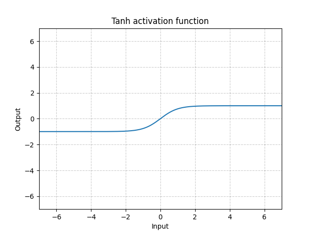
Tanhshrink

Threshold
-
class
torch.nn.Threshold(threshold, value, inplace=False)[source]¶ Thresholds each element of the input Tensor.
Threshold is defined as:
- Parameters
threshold – The value to threshold at
value – The value to replace with
inplace – can optionally do the operation in-place. Default:
False
- Shape:
Input: where * means, any number of additional dimensions
Output: , same shape as the input
Examples:
>>> m = nn.Threshold(0.1, 20)
>>> input = torch.randn(2)
>>> output = m(input)
Non-linear activations (other)
Softmin
-
class
torch.nn.Softmin(dim=None)[source]¶ Applies the Softmin function to an n-dimensional input Tensor rescaling them so that the elements of the n-dimensional output Tensor lie in the range [0, 1] and sum to 1.
Softmin is defined as:
- Shape:
Input: where * means, any number of additional dimensions
Output: , same shape as the input
- Parameters
dim (int) – A dimension along which Softmin will be computed (so every slice along dim will sum to 1).
- Returns
a Tensor of the same dimension and shape as the input, with values in the range [0, 1]
Examples:
>>> m = nn.Softmin()
>>> input = torch.randn(2, 3)
>>> output = m(input)
Softmax
-
class
torch.nn.Softmax(dim=None)[source]¶ Applies the Softmax function to an n-dimensional input Tensor rescaling them so that the elements of the n-dimensional output Tensor lie in the range [0,1] and sum to 1.
Softmax is defined as:
- Shape:
Input: where * means, any number of additional dimensions
Output: , same shape as the input
- Returns
a Tensor of the same dimension and shape as the input with values in the range [0, 1]
- Parameters
dim (int) – A dimension along which Softmax will be computed (so every slice along dim will sum to 1).
Note
This module doesn’t work directly with NLLLoss, which expects the Log to be computed between the Softmax and itself. Use LogSoftmax instead (it’s faster and has better numerical properties).
Examples:
>>> m = nn.Softmax(dim=1)
>>> input = torch.randn(2, 3)
>>> output = m(input)
Softmax2d
-
class
torch.nn.Softmax2d[source]¶ Applies SoftMax over features to each spatial location.
When given an image of
Channels x Height x Width, it will apply Softmax to each location- Shape:
Input:
Output: (same shape as input)
- Returns
a Tensor of the same dimension and shape as the input with values in the range [0, 1]
Examples:
>>> m = nn.Softmax2d()
>>> # you softmax over the 2nd dimension
>>> input = torch.randn(2, 3, 12, 13)
>>> output = m(input)
LogSoftmax
-
class
torch.nn.LogSoftmax(dim=None)[source]¶ Applies the function to an n-dimensional input Tensor. The LogSoftmax formulation can be simplified as:
- Shape:
Input: where * means, any number of additional dimensions
Output: , same shape as the input
- Parameters
dim (int) – A dimension along which LogSoftmax will be computed.
- Returns
a Tensor of the same dimension and shape as the input with values in the range [-inf, 0)
Examples:
>>> m = nn.LogSoftmax()
>>> input = torch.randn(2, 3)
>>> output = m(input)
AdaptiveLogSoftmaxWithLoss
-
class
torch.nn.AdaptiveLogSoftmaxWithLoss(in_features, n_classes, cutoffs, div_value=4.0, head_bias=False)[source]¶ Efficient softmax approximation as described in Efficient softmax approximation for GPUs by Edouard Grave, Armand Joulin, Moustapha Cissé, David Grangier, and Hervé Jégou.
Adaptive softmax is an approximate strategy for training models with large output spaces. It is most effective when the label distribution is highly imbalanced, for example in natural language modelling, where the word frequency distribution approximately follows the Zipf’s law.
Adaptive softmax partitions the labels into several clusters, according to their frequency. These clusters may contain different number of targets each. Additionally, clusters containing less frequent labels assign lower dimensional embeddings to those labels, which speeds up the computation. For each minibatch, only clusters for which at least one target is present are evaluated.
The idea is that the clusters which are accessed frequently (like the first one, containing most frequent labels), should also be cheap to compute – that is, contain a small number of assigned labels.
We highly recommend taking a look at the original paper for more details.
cutoffsshould be an ordered Sequence of integers sorted in the increasing order. It controls number of clusters and the partitioning of targets into clusters. For example settingcutoffs = [10, 100, 1000]means that first 10 targets will be assigned to the ‘head’ of the adaptive softmax, targets 11, 12, …, 100 will be assigned to the first cluster, and targets 101, 102, …, 1000 will be assigned to the second cluster, while targets 1001, 1002, …, n_classes - 1 will be assigned to the last, third cluster.div_valueis used to compute the size of each additional cluster, which is given as , where is the cluster index (with clusters for less frequent words having larger indices, and indices starting from ).head_biasif set to True, adds a bias term to the ‘head’ of the adaptive softmax. See paper for details. Set to False in the official implementation.
Warning
Labels passed as inputs to this module should be sorted according to their frequency. This means that the most frequent label should be represented by the index 0, and the least frequent label should be represented by the index n_classes - 1.
Note
This module returns a
NamedTuplewithoutputandlossfields. See further documentation for details.Note
To compute log-probabilities for all classes, the
log_probmethod can be used.- Parameters
in_features (int) – Number of features in the input tensor
n_classes (int) – Number of classes in the dataset
cutoffs (Sequence) – Cutoffs used to assign targets to their buckets
div_value (float, optional) – value used as an exponent to compute sizes of the clusters. Default: 4.0
head_bias (bool, optional) – If
True, adds a bias term to the ‘head’ of the adaptive softmax. Default:False
- Returns
output is a Tensor of size
Ncontaining computed target log probabilities for each exampleloss is a Scalar representing the computed negative log likelihood loss
- Return type
NamedTuplewithoutputandlossfields
- Shape:
input:
target: where each value satisfies
output1:
output2:
Scalar
Normalization layers
BatchNorm1d
-
class
torch.nn.BatchNorm1d(num_features, eps=1e-05, momentum=0.1, affine=True, track_running_stats=True)[source]¶ Applies Batch Normalization over a 2D or 3D input (a mini-batch of 1D inputs with optional additional channel dimension) as described in the paper Batch Normalization: Accelerating Deep Network Training by Reducing Internal Covariate Shift .
The mean and standard-deviation are calculated per-dimension over the mini-batches and and are learnable parameter vectors of size C (where C is the input size). By default, the elements of are set to 1 and the elements of are set to 0.
Also by default, during training this layer keeps running estimates of its computed mean and variance, which are then used for normalization during evaluation. The running estimates are kept with a default
momentumof 0.1.If
track_running_statsis set toFalse, this layer then does not keep running estimates, and batch statistics are instead used during evaluation time as well.Note
This
momentumargument is different from one used in optimizer classes and the conventional notion of momentum. Mathematically, the update rule for running statistics here is , where is the estimated statistic and is the new observed value.Because the Batch Normalization is done over the C dimension, computing statistics on (N, L) slices, it’s common terminology to call this Temporal Batch Normalization.
- Parameters
num_features – from an expected input of size or from input of size
eps – a value added to the denominator for numerical stability. Default: 1e-5
momentum – the value used for the running_mean and running_var computation. Can be set to
Nonefor cumulative moving average (i.e. simple average). Default: 0.1affine – a boolean value that when set to
True, this module has learnable affine parameters. Default:Truetrack_running_stats – a boolean value that when set to
True, this module tracks the running mean and variance, and when set toFalse, this module does not track such statistics and always uses batch statistics in both training and eval modes. Default:True
- Shape:
Input: or
Output: or (same shape as input)
Examples:
>>> # With Learnable Parameters
>>> m = nn.BatchNorm1d(100)
>>> # Without Learnable Parameters
>>> m = nn.BatchNorm1d(100, affine=False)
>>> input = torch.randn(20, 100)
>>> output = m(input)
BatchNorm2d
-
class
torch.nn.BatchNorm2d(num_features, eps=1e-05, momentum=0.1, affine=True, track_running_stats=True)[source]¶ Applies Batch Normalization over a 4D input (a mini-batch of 2D inputs with additional channel dimension) as described in the paper Batch Normalization: Accelerating Deep Network Training by Reducing Internal Covariate Shift .
The mean and standard-deviation are calculated per-dimension over the mini-batches and and are learnable parameter vectors of size C (where C is the input size). By default, the elements of are set to 1 and the elements of are set to 0.
Also by default, during training this layer keeps running estimates of its computed mean and variance, which are then used for normalization during evaluation. The running estimates are kept with a default
momentumof 0.1.If
track_running_statsis set toFalse, this layer then does not keep running estimates, and batch statistics are instead used during evaluation time as well.Note
This
momentumargument is different from one used in optimizer classes and the conventional notion of momentum. Mathematically, the update rule for running statistics here is , where is the estimated statistic and is the new observed value.Because the Batch Normalization is done over the C dimension, computing statistics on (N, H, W) slices, it’s common terminology to call this Spatial Batch Normalization.
- Parameters
num_features – from an expected input of size
eps – a value added to the denominator for numerical stability. Default: 1e-5
momentum – the value used for the running_mean and running_var computation. Can be set to
Nonefor cumulative moving average (i.e. simple average). Default: 0.1affine – a boolean value that when set to
True, this module has learnable affine parameters. Default:Truetrack_running_stats – a boolean value that when set to
True, this module tracks the running mean and variance, and when set toFalse, this module does not track such statistics and always uses batch statistics in both training and eval modes. Default:True
- Shape:
Input:
Output: (same shape as input)
Examples:
>>> # With Learnable Parameters
>>> m = nn.BatchNorm2d(100)
>>> # Without Learnable Parameters
>>> m = nn.BatchNorm2d(100, affine=False)
>>> input = torch.randn(20, 100, 35, 45)
>>> output = m(input)
BatchNorm3d
-
class
torch.nn.BatchNorm3d(num_features, eps=1e-05, momentum=0.1, affine=True, track_running_stats=True)[source]¶ Applies Batch Normalization over a 5D input (a mini-batch of 3D inputs with additional channel dimension) as described in the paper Batch Normalization: Accelerating Deep Network Training by Reducing Internal Covariate Shift .
The mean and standard-deviation are calculated per-dimension over the mini-batches and and are learnable parameter vectors of size C (where C is the input size). By default, the elements of are set to 1 and the elements of are set to 0.
Also by default, during training this layer keeps running estimates of its computed mean and variance, which are then used for normalization during evaluation. The running estimates are kept with a default
momentumof 0.1.If
track_running_statsis set toFalse, this layer then does not keep running estimates, and batch statistics are instead used during evaluation time as well.Note
This
momentumargument is different from one used in optimizer classes and the conventional notion of momentum. Mathematically, the update rule for running statistics here is , where is the estimated statistic and is the new observed value.Because the Batch Normalization is done over the C dimension, computing statistics on (N, D, H, W) slices, it’s common terminology to call this Volumetric Batch Normalization or Spatio-temporal Batch Normalization.
- Parameters
num_features – from an expected input of size
eps – a value added to the denominator for numerical stability. Default: 1e-5
momentum – the value used for the running_mean and running_var computation. Can be set to
Nonefor cumulative moving average (i.e. simple average). Default: 0.1affine – a boolean value that when set to
True, this module has learnable affine parameters. Default:Truetrack_running_stats – a boolean value that when set to
True, this module tracks the running mean and variance, and when set toFalse, this module does not track such statistics and always uses batch statistics in both training and eval modes. Default:True
- Shape:
Input:
Output: (same shape as input)
Examples:
>>> # With Learnable Parameters
>>> m = nn.BatchNorm3d(100)
>>> # Without Learnable Parameters
>>> m = nn.BatchNorm3d(100, affine=False)
>>> input = torch.randn(20, 100, 35, 45, 10)
>>> output = m(input)
GroupNorm
-
class
torch.nn.GroupNorm(num_groups, num_channels, eps=1e-05, affine=True)[source]¶ Applies Group Normalization over a mini-batch of inputs as described in the paper Group Normalization .
The input channels are separated into
num_groupsgroups, each containingnum_channels / num_groupschannels. The mean and standard-deviation are calculated separately over the each group. and are learnable per-channel affine transform parameter vectors of sizenum_channelsifaffineisTrue.This layer uses statistics computed from input data in both training and evaluation modes.
- Parameters
num_groups (int) – number of groups to separate the channels into
num_channels (int) – number of channels expected in input
eps – a value added to the denominator for numerical stability. Default: 1e-5
affine – a boolean value that when set to
True, this module has learnable per-channel affine parameters initialized to ones (for weights) and zeros (for biases). Default:True.
- Shape:
Input: where
Output: (same shape as input)
Examples:
>>> input = torch.randn(20, 6, 10, 10)
>>> # Separate 6 channels into 3 groups
>>> m = nn.GroupNorm(3, 6)
>>> # Separate 6 channels into 6 groups (equivalent with InstanceNorm)
>>> m = nn.GroupNorm(6, 6)
>>> # Put all 6 channels into a single group (equivalent with LayerNorm)
>>> m = nn.GroupNorm(1, 6)
>>> # Activating the module
>>> output = m(input)
SyncBatchNorm
-
class
torch.nn.SyncBatchNorm(num_features, eps=1e-05, momentum=0.1, affine=True, track_running_stats=True, process_group=None)[source]¶ Applies Batch Normalization over a N-Dimensional input (a mini-batch of [N-2]D inputs with additional channel dimension) as described in the paper Batch Normalization: Accelerating Deep Network Training by Reducing Internal Covariate Shift .
The mean and standard-deviation are calculated per-dimension over all mini-batches of the same process groups. and are learnable parameter vectors of size C (where C is the input size). By default, the elements of are sampled from and the elements of are set to 0.
Also by default, during training this layer keeps running estimates of its computed mean and variance, which are then used for normalization during evaluation. The running estimates are kept with a default
momentumof 0.1.If
track_running_statsis set toFalse, this layer then does not keep running estimates, and batch statistics are instead used during evaluation time as well.Note
This
momentumargument is different from one used in optimizer classes and the conventional notion of momentum. Mathematically, the update rule for running statistics here is , where is the estimated statistic and is the new observed value.Because the Batch Normalization is done over the C dimension, computing statistics on (N, +) slices, it’s common terminology to call this Volumetric Batch Normalization or Spatio-temporal Batch Normalization.
Currently SyncBatchNorm only supports DistributedDataParallel with single GPU per process. Use torch.nn.SyncBatchNorm.convert_sync_batchnorm() to convert BatchNorm layer to SyncBatchNorm before wrapping Network with DDP.
- Parameters
num_features – from an expected input of size
eps – a value added to the denominator for numerical stability. Default: 1e-5
momentum – the value used for the running_mean and running_var computation. Can be set to
Nonefor cumulative moving average (i.e. simple average). Default: 0.1affine – a boolean value that when set to
True, this module has learnable affine parameters. Default:Truetrack_running_stats – a boolean value that when set to
True, this module tracks the running mean and variance, and when set toFalse, this module does not track such statistics and always uses batch statistics in both training and eval modes. Default:Trueprocess_group – synchronization of stats happen within each process group individually. Default behavior is synchronization across the whole world
- Shape:
Input:
Output: (same shape as input)
Examples:
>>> # With Learnable Parameters
>>> m = nn.SyncBatchNorm(100)
>>> # creating process group (optional)
>>> # process_ids is a list of int identifying rank ids.
>>> process_group = torch.distributed.new_group(process_ids)
>>> # Without Learnable Parameters
>>> m = nn.BatchNorm3d(100, affine=False, process_group=process_group)
>>> input = torch.randn(20, 100, 35, 45, 10)
>>> output = m(input)

>>> # network is nn.BatchNorm layer
>>> sync_bn_network = nn.SyncBatchNorm.convert_sync_batchnorm(network, process_group)
>>> # only single gpu per process is currently supported
>>> ddp_sync_bn_network = torch.nn.parallel.DistributedDataParallel(
>>>                         sync_bn_network,
>>>                         device_ids=[args.local_rank],
>>>                         output_device=args.local_rank)
-
classmethod
convert_sync_batchnorm(module, process_group=None)[source]¶ Helper function to convert torch.nn.BatchNormND layer in the model to torch.nn.SyncBatchNorm layer.
- Parameters
module (nn.Module) – containing module
process_group (optional) – process group to scope synchronization,
default is the whole world
- Returns
The original module with the converted torch.nn.SyncBatchNorm layer
Example:
>>> # Network with nn.BatchNorm layer
>>> module = torch.nn.Sequential(
>>>            torch.nn.Linear(20, 100),
>>>            torch.nn.BatchNorm1d(100)
>>>          ).cuda()
>>> # creating process group (optional)
>>> # process_ids is a list of int identifying rank ids.
>>> process_group = torch.distributed.new_group(process_ids)
>>> sync_bn_module = convert_sync_batchnorm(module, process_group)
InstanceNorm1d
-
class
torch.nn.InstanceNorm1d(num_features, eps=1e-05, momentum=0.1, affine=False, track_running_stats=False)[source]¶ Applies Instance Normalization over a 3D input (a mini-batch of 1D inputs with optional additional channel dimension) as described in the paper Instance Normalization: The Missing Ingredient for Fast Stylization .
The mean and standard-deviation are calculated per-dimension separately for each object in a mini-batch. and are learnable parameter vectors of size C (where C is the input size) if
affineisTrue.By default, this layer uses instance statistics computed from input data in both training and evaluation modes.
If
track_running_statsis set toTrue, during training this layer keeps running estimates of its computed mean and variance, which are then used for normalization during evaluation. The running estimates are kept with a defaultmomentumof 0.1.Note
This
momentumargument is different from one used in optimizer classes and the conventional notion of momentum. Mathematically, the update rule for running statistics here is , where is the estimated statistic and is the new observed value.Note
InstanceNorm1dandLayerNormare very similar, but have some subtle differences.InstanceNorm1dis applied on each channel of channeled data like multidimensional time series, butLayerNormis usually applied on entire sample and often in NLP tasks. Additionally,LayerNormapplies elementwise affine transform, whileInstanceNorm1dusually don’t apply affine transform.- Parameters
num_features – from an expected input of size or from input of size
eps – a value added to the denominator for numerical stability. Default: 1e-5
momentum – the value used for the running_mean and running_var computation. Default: 0.1
affine – a boolean value that when set to
True, this module has learnable affine parameters, initialized the same way as done for batch normalization. Default:False.track_running_stats – a boolean value that when set to
True, this module tracks the running mean and variance, and when set toFalse, this module does not track such statistics and always uses batch statistics in both training and eval modes. Default:False
- Shape:
Input:
Output: (same shape as input)
Examples:
>>> # Without Learnable Parameters
>>> m = nn.InstanceNorm1d(100)
>>> # With Learnable Parameters
>>> m = nn.InstanceNorm1d(100, affine=True)
>>> input = torch.randn(20, 100, 40)
>>> output = m(input)
InstanceNorm2d
-
class
torch.nn.InstanceNorm2d(num_features, eps=1e-05, momentum=0.1, affine=False, track_running_stats=False)[source]¶ Applies Instance Normalization over a 4D input (a mini-batch of 2D inputs with additional channel dimension) as described in the paper Instance Normalization: The Missing Ingredient for Fast Stylization .
The mean and standard-deviation are calculated per-dimension separately for each object in a mini-batch. and are learnable parameter vectors of size C (where C is the input size) if
affineisTrue.By default, this layer uses instance statistics computed from input data in both training and evaluation modes.
If
track_running_statsis set toTrue, during training this layer keeps running estimates of its computed mean and variance, which are then used for normalization during evaluation. The running estimates are kept with a defaultmomentumof 0.1.Note
This
momentumargument is different from one used in optimizer classes and the conventional notion of momentum. Mathematically, the update rule for running statistics here is , where is the estimated statistic and is the new observed value.Note
InstanceNorm2dandLayerNormare very similar, but have some subtle differences.InstanceNorm2dis applied on each channel of channeled data like RGB images, butLayerNormis usually applied on entire sample and often in NLP tasks. Additionally,LayerNormapplies elementwise affine transform, whileInstanceNorm2dusually don’t apply affine transform.- Parameters
num_features – from an expected input of size
eps – a value added to the denominator for numerical stability. Default: 1e-5
momentum – the value used for the running_mean and running_var computation. Default: 0.1
affine – a boolean value that when set to
True, this module has learnable affine parameters, initialized the same way as done for batch normalization. Default:False.track_running_stats – a boolean value that when set to
True, this module tracks the running mean and variance, and when set toFalse, this module does not track such statistics and always uses batch statistics in both training and eval modes. Default:False
- Shape:
Input:
Output: (same shape as input)
Examples:
>>> # Without Learnable Parameters
>>> m = nn.InstanceNorm2d(100)
>>> # With Learnable Parameters
>>> m = nn.InstanceNorm2d(100, affine=True)
>>> input = torch.randn(20, 100, 35, 45)
>>> output = m(input)
InstanceNorm3d
-
class
torch.nn.InstanceNorm3d(num_features, eps=1e-05, momentum=0.1, affine=False, track_running_stats=False)[source]¶ Applies Instance Normalization over a 5D input (a mini-batch of 3D inputs with additional channel dimension) as described in the paper Instance Normalization: The Missing Ingredient for Fast Stylization .
The mean and standard-deviation are calculated per-dimension separately for each object in a mini-batch. and are learnable parameter vectors of size C (where C is the input size) if
affineisTrue.By default, this layer uses instance statistics computed from input data in both training and evaluation modes.
If
track_running_statsis set toTrue, during training this layer keeps running estimates of its computed mean and variance, which are then used for normalization during evaluation. The running estimates are kept with a defaultmomentumof 0.1.Note
This
momentumargument is different from one used in optimizer classes and the conventional notion of momentum. Mathematically, the update rule for running statistics here is , where is the estimated statistic and is the new observed value.Note
InstanceNorm3dandLayerNormare very similar, but have some subtle differences.InstanceNorm3dis applied on each channel of channeled data like 3D models with RGB color, butLayerNormis usually applied on entire sample and often in NLP tasks. Additionally,LayerNormapplies elementwise affine transform, whileInstanceNorm3dusually don’t apply affine transform.- Parameters
num_features – from an expected input of size
eps – a value added to the denominator for numerical stability. Default: 1e-5
momentum – the value used for the running_mean and running_var computation. Default: 0.1
affine – a boolean value that when set to
True, this module has learnable affine parameters, initialized the same way as done for batch normalization. Default:False.track_running_stats – a boolean value that when set to
True, this module tracks the running mean and variance, and when set toFalse, this module does not track such statistics and always uses batch statistics in both training and eval modes. Default:False
- Shape:
Input:
Output: (same shape as input)
Examples:
>>> # Without Learnable Parameters
>>> m = nn.InstanceNorm3d(100)
>>> # With Learnable Parameters
>>> m = nn.InstanceNorm3d(100, affine=True)
>>> input = torch.randn(20, 100, 35, 45, 10)
>>> output = m(input)
LayerNorm
-
class
torch.nn.LayerNorm(normalized_shape, eps=1e-05, elementwise_affine=True)[source]¶ Applies Layer Normalization over a mini-batch of inputs as described in the paper Layer Normalization .
The mean and standard-deviation are calculated separately over the last certain number dimensions which have to be of the shape specified by
normalized_shape. and are learnable affine transform parameters ofnormalized_shapeifelementwise_affineisTrue.Note
Unlike Batch Normalization and Instance Normalization, which applies scalar scale and bias for each entire channel/plane with the
affineoption, Layer Normalization applies per-element scale and bias withelementwise_affine.This layer uses statistics computed from input data in both training and evaluation modes.
- Parameters
normalized_shape (int or list or torch.Size) –
input shape from an expected input of size
If a single integer is used, it is treated as a singleton list, and this module will normalize over the last dimension which is expected to be of that specific size.
eps – a value added to the denominator for numerical stability. Default: 1e-5
elementwise_affine – a boolean value that when set to
True, this module has learnable per-element affine parameters initialized to ones (for weights) and zeros (for biases). Default:True.
- Shape:
Input:
Output: (same shape as input)
Examples:
>>> input = torch.randn(20, 5, 10, 10)
>>> # With Learnable Parameters
>>> m = nn.LayerNorm(input.size()[1:])
>>> # Without Learnable Parameters
>>> m = nn.LayerNorm(input.size()[1:], elementwise_affine=False)
>>> # Normalize over last two dimensions
>>> m = nn.LayerNorm([10, 10])
>>> # Normalize over last dimension of size 10
>>> m = nn.LayerNorm(10)
>>> # Activating the module
>>> output = m(input)
LocalResponseNorm
-
class
torch.nn.LocalResponseNorm(size, alpha=0.0001, beta=0.75, k=1.0)[source]¶ Applies local response normalization over an input signal composed of several input planes, where channels occupy the second dimension. Applies normalization across channels.
- Parameters
size – amount of neighbouring channels used for normalization
alpha – multiplicative factor. Default: 0.0001
beta – exponent. Default: 0.75
k – additive factor. Default: 1
- Shape:
Input:
Output: (same shape as input)
Examples:
>>> lrn = nn.LocalResponseNorm(2)
>>> signal_2d = torch.randn(32, 5, 24, 24)
>>> signal_4d = torch.randn(16, 5, 7, 7, 7, 7)
>>> output_2d = lrn(signal_2d)
>>> output_4d = lrn(signal_4d)
Recurrent layers
RNNBase
RNN
-
class
torch.nn.RNN(*args, **kwargs)[source]¶ Applies a multi-layer Elman RNN with or non-linearity to an input sequence.
For each element in the input sequence, each layer computes the following function:
where is the hidden state at time t, is the input at time t, and is the hidden state of the previous layer at time t-1 or the initial hidden state at time 0. If
nonlinearityis'relu', then is used instead of .- Parameters
input_size – The number of expected features in the input x
hidden_size – The number of features in the hidden state h
num_layers – Number of recurrent layers. E.g., setting
num_layers=2would mean stacking two RNNs together to form a stacked RNN, with the second RNN taking in outputs of the first RNN and computing the final results. Default: 1nonlinearity – The non-linearity to use. Can be either
'tanh'or'relu'. Default:'tanh'bias – If
False, then the layer does not use bias weights b_ih and b_hh. Default:Truebatch_first – If
True, then the input and output tensors are provided as (batch, seq, feature). Default:Falsedropout – If non-zero, introduces a Dropout layer on the outputs of each RNN layer except the last layer, with dropout probability equal to
dropout. Default: 0bidirectional – If
True, becomes a bidirectional RNN. Default:False
- Inputs: input, h_0
input of shape (seq_len, batch, input_size): tensor containing the features of the input sequence. The input can also be a packed variable length sequence. See
torch.nn.utils.rnn.pack_padded_sequence()ortorch.nn.utils.rnn.pack_sequence()for details.h_0 of shape (num_layers * num_directions, batch, hidden_size): tensor containing the initial hidden state for each element in the batch. Defaults to zero if not provided. If the RNN is bidirectional, num_directions should be 2, else it should be 1.
- Outputs: output, h_n
output of shape (seq_len, batch, num_directions * hidden_size): tensor containing the output features (h_t) from the last layer of the RNN, for each t. If a
torch.nn.utils.rnn.PackedSequencehas been given as the input, the output will also be a packed sequence.For the unpacked case, the directions can be separated using
output.view(seq_len, batch, num_directions, hidden_size), with forward and backward being direction 0 and 1 respectively. Similarly, the directions can be separated in the packed case.h_n of shape (num_layers * num_directions, batch, hidden_size): tensor containing the hidden state for t = seq_len.
Like output, the layers can be separated using
h_n.view(num_layers, num_directions, batch, hidden_size).
- Shape:
Input1: tensor containing input features where and L represents a sequence length.
Input2: tensor containing the initial hidden state for each element in the batch. Defaults to zero if not provided. where If the RNN is bidirectional, num_directions should be 2, else it should be 1.
Output1: where
Output2: tensor containing the next hidden state for each element in the batch
- Variables
~RNN.weight_ih_l[k] – the learnable input-hidden weights of the k-th layer, of shape (hidden_size, input_size) for k = 0. Otherwise, the shape is (hidden_size, num_directions * hidden_size)
~RNN.weight_hh_l[k] – the learnable hidden-hidden weights of the k-th layer, of shape (hidden_size, hidden_size)
~RNN.bias_ih_l[k] – the learnable input-hidden bias of the k-th layer, of shape (hidden_size)
~RNN.bias_hh_l[k] – the learnable hidden-hidden bias of the k-th layer, of shape (hidden_size)
Note
All the weights and biases are initialized from where
Note
If the following conditions are satisfied: 1) cudnn is enabled, 2) input data is on the GPU 3) input data has dtype
torch.float164) V100 GPU is used, 5) input data is not inPackedSequenceformat persistent algorithm can be selected to improve performance.Examples:
>>> rnn = nn.RNN(10, 20, 2)
>>> input = torch.randn(5, 3, 10)
>>> h0 = torch.randn(2, 3, 20)
>>> output, hn = rnn(input, h0)
LSTM
-
class
torch.nn.LSTM(*args, **kwargs)[source]¶ Applies a multi-layer long short-term memory (LSTM) RNN to an input sequence.
For each element in the input sequence, each layer computes the following function:
where is the hidden state at time t, is the cell state at time t, is the input at time t, is the hidden state of the layer at time t-1 or the initial hidden state at time 0, and , , , are the input, forget, cell, and output gates, respectively. is the sigmoid function, and is the Hadamard product.
In a multilayer LSTM, the input of the -th layer ( ) is the hidden state of the previous layer multiplied by dropout where each is a Bernoulli random variable which is with probability
dropout.- Parameters
input_size – The number of expected features in the input x
hidden_size – The number of features in the hidden state h
num_layers – Number of recurrent layers. E.g., setting
num_layers=2would mean stacking two LSTMs together to form a stacked LSTM, with the second LSTM taking in outputs of the first LSTM and computing the final results. Default: 1bias – If
False, then the layer does not use bias weights b_ih and b_hh. Default:Truebatch_first – If
True, then the input and output tensors are provided as (batch, seq, feature). Default:Falsedropout – If non-zero, introduces a Dropout layer on the outputs of each LSTM layer except the last layer, with dropout probability equal to
dropout. Default: 0bidirectional – If
True, becomes a bidirectional LSTM. Default:False
- Inputs: input, (h_0, c_0)
input of shape (seq_len, batch, input_size): tensor containing the features of the input sequence. The input can also be a packed variable length sequence. See
torch.nn.utils.rnn.pack_padded_sequence()ortorch.nn.utils.rnn.pack_sequence()for details.h_0 of shape (num_layers * num_directions, batch, hidden_size): tensor containing the initial hidden state for each element in the batch. If the LSTM is bidirectional, num_directions should be 2, else it should be 1.
c_0 of shape (num_layers * num_directions, batch, hidden_size): tensor containing the initial cell state for each element in the batch.
If (h_0, c_0) is not provided, both h_0 and c_0 default to zero.
- Outputs: output, (h_n, c_n)
output of shape (seq_len, batch, num_directions * hidden_size): tensor containing the output features (h_t) from the last layer of the LSTM, for each t. If a
torch.nn.utils.rnn.PackedSequencehas been given as the input, the output will also be a packed sequence.For the unpacked case, the directions can be separated using
output.view(seq_len, batch, num_directions, hidden_size), with forward and backward being direction 0 and 1 respectively. Similarly, the directions can be separated in the packed case.h_n of shape (num_layers * num_directions, batch, hidden_size): tensor containing the hidden state for t = seq_len.
Like output, the layers can be separated using
h_n.view(num_layers, num_directions, batch, hidden_size)and similarly for c_n.c_n of shape (num_layers * num_directions, batch, hidden_size): tensor containing the cell state for t = seq_len.
- Variables
~LSTM.weight_ih_l[k] – the learnable input-hidden weights of the layer (W_ii|W_if|W_ig|W_io), of shape (4*hidden_size, input_size) for k = 0. Otherwise, the shape is (4*hidden_size, num_directions * hidden_size)
~LSTM.weight_hh_l[k] – the learnable hidden-hidden weights of the layer (W_hi|W_hf|W_hg|W_ho), of shape (4*hidden_size, hidden_size)
~LSTM.bias_ih_l[k] – the learnable input-hidden bias of the layer (b_ii|b_if|b_ig|b_io), of shape (4*hidden_size)
~LSTM.bias_hh_l[k] – the learnable hidden-hidden bias of the layer (b_hi|b_hf|b_hg|b_ho), of shape (4*hidden_size)
Note
All the weights and biases are initialized from where
Note
If the following conditions are satisfied: 1) cudnn is enabled, 2) input data is on the GPU 3) input data has dtype
torch.float164) V100 GPU is used, 5) input data is not inPackedSequenceformat persistent algorithm can be selected to improve performance.Examples:
>>> rnn = nn.LSTM(10, 20, 2)
>>> input = torch.randn(5, 3, 10)
>>> h0 = torch.randn(2, 3, 20)
>>> c0 = torch.randn(2, 3, 20)
>>> output, (hn, cn) = rnn(input, (h0, c0))
GRU
-
class
torch.nn.GRU(*args, **kwargs)[source]¶ Applies a multi-layer gated recurrent unit (GRU) RNN to an input sequence.
For each element in the input sequence, each layer computes the following function:
where is the hidden state at time t, is the input at time t, is the hidden state of the layer at time t-1 or the initial hidden state at time 0, and , , are the reset, update, and new gates, respectively. is the sigmoid function, and is the Hadamard product.
In a multilayer GRU, the input of the -th layer ( ) is the hidden state of the previous layer multiplied by dropout where each is a Bernoulli random variable which is with probability
dropout.- Parameters
input_size – The number of expected features in the input x
hidden_size – The number of features in the hidden state h
num_layers – Number of recurrent layers. E.g., setting
num_layers=2would mean stacking two GRUs together to form a stacked GRU, with the second GRU taking in outputs of the first GRU and computing the final results. Default: 1bias – If
False, then the layer does not use bias weights b_ih and b_hh. Default:Truebatch_first – If
True, then the input and output tensors are provided as (batch, seq, feature). Default:Falsedropout – If non-zero, introduces a Dropout layer on the outputs of each GRU layer except the last layer, with dropout probability equal to
dropout. Default: 0bidirectional – If
True, becomes a bidirectional GRU. Default:False
- Inputs: input, h_0
input of shape (seq_len, batch, input_size): tensor containing the features of the input sequence. The input can also be a packed variable length sequence. See
torch.nn.utils.rnn.pack_padded_sequence()for details.h_0 of shape (num_layers * num_directions, batch, hidden_size): tensor containing the initial hidden state for each element in the batch. Defaults to zero if not provided. If the RNN is bidirectional, num_directions should be 2, else it should be 1.
- Outputs: output, h_n
output of shape (seq_len, batch, num_directions * hidden_size): tensor containing the output features h_t from the last layer of the GRU, for each t. If a
torch.nn.utils.rnn.PackedSequencehas been given as the input, the output will also be a packed sequence. For the unpacked case, the directions can be separated usingoutput.view(seq_len, batch, num_directions, hidden_size), with forward and backward being direction 0 and 1 respectively.Similarly, the directions can be separated in the packed case.
h_n of shape (num_layers * num_directions, batch, hidden_size): tensor containing the hidden state for t = seq_len
Like output, the layers can be separated using
h_n.view(num_layers, num_directions, batch, hidden_size).
- Shape:
Input1: tensor containing input features where and L represents a sequence length.
Input2: tensor containing the initial hidden state for each element in the batch. Defaults to zero if not provided. where If the RNN is bidirectional, num_directions should be 2, else it should be 1.
Output1: where
Output2: tensor containing the next hidden state for each element in the batch
- Variables
~GRU.weight_ih_l[k] – the learnable input-hidden weights of the layer (W_ir|W_iz|W_in), of shape (3*hidden_size, input_size) for k = 0. Otherwise, the shape is (3*hidden_size, num_directions * hidden_size)
~GRU.weight_hh_l[k] – the learnable hidden-hidden weights of the layer (W_hr|W_hz|W_hn), of shape (3*hidden_size, hidden_size)
~GRU.bias_ih_l[k] – the learnable input-hidden bias of the layer (b_ir|b_iz|b_in), of shape (3*hidden_size)
~GRU.bias_hh_l[k] – the learnable hidden-hidden bias of the layer (b_hr|b_hz|b_hn), of shape (3*hidden_size)
Note
All the weights and biases are initialized from where
Note
If the following conditions are satisfied: 1) cudnn is enabled, 2) input data is on the GPU 3) input data has dtype
torch.float164) V100 GPU is used, 5) input data is not inPackedSequenceformat persistent algorithm can be selected to improve performance.Examples:
>>> rnn = nn.GRU(10, 20, 2)
>>> input = torch.randn(5, 3, 10)
>>> h0 = torch.randn(2, 3, 20)
>>> output, hn = rnn(input, h0)
RNNCell
-
class
torch.nn.RNNCell(input_size, hidden_size, bias=True, nonlinearity='tanh')[source]¶ An Elman RNN cell with tanh or ReLU non-linearity.
If
nonlinearityis ‘relu’, then ReLU is used in place of tanh.- Parameters
input_size – The number of expected features in the input x
hidden_size – The number of features in the hidden state h
bias – If
False, then the layer does not use bias weights b_ih and b_hh. Default:Truenonlinearity – The non-linearity to use. Can be either
'tanh'or'relu'. Default:'tanh'
- Inputs: input, hidden
input of shape (batch, input_size): tensor containing input features
hidden of shape (batch, hidden_size): tensor containing the initial hidden state for each element in the batch. Defaults to zero if not provided.
- Outputs: h’
h’ of shape (batch, hidden_size): tensor containing the next hidden state for each element in the batch
- Shape:
Input1: tensor containing input features where = input_size
Input2: tensor containing the initial hidden state for each element in the batch where = hidden_size Defaults to zero if not provided.
Output: tensor containing the next hidden state for each element in the batch
- Variables
~RNNCell.weight_ih – the learnable input-hidden weights, of shape (hidden_size, input_size)
~RNNCell.weight_hh – the learnable hidden-hidden weights, of shape (hidden_size, hidden_size)
~RNNCell.bias_ih – the learnable input-hidden bias, of shape (hidden_size)
~RNNCell.bias_hh – the learnable hidden-hidden bias, of shape (hidden_size)
Note
All the weights and biases are initialized from where
Examples:
>>> rnn = nn.RNNCell(10, 20)
>>> input = torch.randn(6, 3, 10)
>>> hx = torch.randn(3, 20)
>>> output = []
>>> for i in range(6):
        hx = rnn(input[i], hx)
        output.append(hx)
LSTMCell
-
class
torch.nn.LSTMCell(input_size, hidden_size, bias=True)[source]¶ A long short-term memory (LSTM) cell.
where is the sigmoid function, and is the Hadamard product.
- Parameters
input_size – The number of expected features in the input x
hidden_size – The number of features in the hidden state h
bias – If
False, then the layer does not use bias weights b_ih and b_hh. Default:True
- Inputs: input, (h_0, c_0)
input of shape (batch, input_size): tensor containing input features
h_0 of shape (batch, hidden_size): tensor containing the initial hidden state for each element in the batch.
c_0 of shape (batch, hidden_size): tensor containing the initial cell state for each element in the batch.
If (h_0, c_0) is not provided, both h_0 and c_0 default to zero.
- Outputs: (h_1, c_1)
h_1 of shape (batch, hidden_size): tensor containing the next hidden state for each element in the batch
c_1 of shape (batch, hidden_size): tensor containing the next cell state for each element in the batch
- Variables
~LSTMCell.weight_ih – the learnable input-hidden weights, of shape (4*hidden_size, input_size)
~LSTMCell.weight_hh – the learnable hidden-hidden weights, of shape (4*hidden_size, hidden_size)
~LSTMCell.bias_ih – the learnable input-hidden bias, of shape (4*hidden_size)
~LSTMCell.bias_hh – the learnable hidden-hidden bias, of shape (4*hidden_size)
Note
All the weights and biases are initialized from where
Examples:
>>> rnn = nn.LSTMCell(10, 20)
>>> input = torch.randn(6, 3, 10)
>>> hx = torch.randn(3, 20)
>>> cx = torch.randn(3, 20)
>>> output = []
>>> for i in range(6):
        hx, cx = rnn(input[i], (hx, cx))
        output.append(hx)
GRUCell
-
class
torch.nn.GRUCell(input_size, hidden_size, bias=True)[source]¶ A gated recurrent unit (GRU) cell
where is the sigmoid function, and is the Hadamard product.
- Parameters
input_size – The number of expected features in the input x
hidden_size – The number of features in the hidden state h
bias – If
False, then the layer does not use bias weights b_ih and b_hh. Default:True
- Inputs: input, hidden
input of shape (batch, input_size): tensor containing input features
hidden of shape (batch, hidden_size): tensor containing the initial hidden state for each element in the batch. Defaults to zero if not provided.
- Outputs: h’
h’ of shape (batch, hidden_size): tensor containing the next hidden state for each element in the batch
- Shape:
Input1: tensor containing input features where = input_size
Input2: tensor containing the initial hidden state for each element in the batch where = hidden_size Defaults to zero if not provided.
Output: tensor containing the next hidden state for each element in the batch
- Variables
~GRUCell.weight_ih – the learnable input-hidden weights, of shape (3*hidden_size, input_size)
~GRUCell.weight_hh – the learnable hidden-hidden weights, of shape (3*hidden_size, hidden_size)
~GRUCell.bias_ih – the learnable input-hidden bias, of shape (3*hidden_size)
~GRUCell.bias_hh – the learnable hidden-hidden bias, of shape (3*hidden_size)
Note
All the weights and biases are initialized from where
Examples:
>>> rnn = nn.GRUCell(10, 20)
>>> input = torch.randn(6, 3, 10)
>>> hx = torch.randn(3, 20)
>>> output = []
>>> for i in range(6):
        hx = rnn(input[i], hx)
        output.append(hx)
Transformer layers
Transformer
-
class
torch.nn.Transformer(d_model=512, nhead=8, num_encoder_layers=6, num_decoder_layers=6, dim_feedforward=2048, dropout=0.1, activation='relu', custom_encoder=None, custom_decoder=None)[source]¶ A transformer model. User is able to modify the attributes as needed. The architecture is based on the paper “Attention Is All You Need”. Ashish Vaswani, Noam Shazeer, Niki Parmar, Jakob Uszkoreit, Llion Jones, Aidan N Gomez, Lukasz Kaiser, and Illia Polosukhin. 2017. Attention is all you need. In Advances in Neural Information Processing Systems, pages 6000-6010. Users can build the BERT(https://arxiv.org/abs/1810.04805) model with corresponding parameters.
- Parameters
d_model – the number of expected features in the encoder/decoder inputs (default=512).
nhead – the number of heads in the multiheadattention models (default=8).
num_encoder_layers – the number of sub-encoder-layers in the encoder (default=6).
num_decoder_layers – the number of sub-decoder-layers in the decoder (default=6).
dim_feedforward – the dimension of the feedforward network model (default=2048).
dropout – the dropout value (default=0.1).
activation – the activation function of encoder/decoder intermediate layer, relu or gelu (default=relu).
custom_encoder – custom encoder (default=None).
custom_decoder – custom decoder (default=None).
- Examples::
>>> transformer_model = nn.Transformer(nhead=16, num_encoder_layers=12)
>>> src = torch.rand((10, 32, 512))
>>> tgt = torch.rand((20, 32, 512))
>>> out = transformer_model(src, tgt)
Note: A full example to apply nn.Transformer module for the word language model is available in https://github.com/pytorch/examples/tree/master/word_language_model
-
forward(src, tgt, src_mask=None, tgt_mask=None, memory_mask=None, src_key_padding_mask=None, tgt_key_padding_mask=None, memory_key_padding_mask=None)[source]¶ Take in and process masked source/target sequences.
- Parameters
src – the sequence to the encoder (required).
tgt – the sequence to the decoder (required).
src_mask – the additive mask for the src sequence (optional).
tgt_mask – the additive mask for the tgt sequence (optional).
memory_mask – the additive mask for the encoder output (optional).
src_key_padding_mask – the ByteTensor mask for src keys per batch (optional).
tgt_key_padding_mask – the ByteTensor mask for tgt keys per batch (optional).
memory_key_padding_mask – the ByteTensor mask for memory keys per batch (optional).
- Shape:
src: .
tgt: .
src_mask: .
tgt_mask: .
memory_mask: .
src_key_padding_mask: .
tgt_key_padding_mask: .
memory_key_padding_mask: .
Note: [src/tgt/memory]_mask should be filled with float(‘-inf’) for the masked positions and float(0.0) else. These masks ensure that predictions for position i depend only on the unmasked positions j and are applied identically for each sequence in a batch. [src/tgt/memory]_key_padding_mask should be a ByteTensor where True values are positions that should be masked with float(‘-inf’) and False values will be unchanged. This mask ensures that no information will be taken from position i if it is masked, and has a separate mask for each sequence in a batch.
output: .
Note: Due to the multi-head attention architecture in the transformer model, the output sequence length of a transformer is same as the input sequence (i.e. target) length of the decode.
where S is the source sequence length, T is the target sequence length, N is the batch size, E is the feature number
Examples
>>> output = transformer_model(src, tgt, src_mask=src_mask, tgt_mask=tgt_mask)
TransformerEncoder
-
class
torch.nn.TransformerEncoder(encoder_layer, num_layers, norm=None)[source]¶ TransformerEncoder is a stack of N encoder layers
- Parameters
encoder_layer – an instance of the TransformerEncoderLayer() class (required).
num_layers – the number of sub-encoder-layers in the encoder (required).
norm – the layer normalization component (optional).
- Examples::
>>> encoder_layer = nn.TransformerEncoderLayer(d_model=512, nhead=8)
>>> transformer_encoder = nn.TransformerEncoder(encoder_layer, num_layers=6)
>>> src = torch.rand(10, 32, 512)
>>> out = transformer_encoder(src)
-
forward(src, mask=None, src_key_padding_mask=None)[source]¶ Pass the input through the encoder layers in turn.
- Parameters
src – the sequence to the encoder (required).
mask – the mask for the src sequence (optional).
src_key_padding_mask – the mask for the src keys per batch (optional).
- Shape:
see the docs in Transformer class.
TransformerDecoder
-
class
torch.nn.TransformerDecoder(decoder_layer, num_layers, norm=None)[source]¶ TransformerDecoder is a stack of N decoder layers
- Parameters
decoder_layer – an instance of the TransformerDecoderLayer() class (required).
num_layers – the number of sub-decoder-layers in the decoder (required).
norm – the layer normalization component (optional).
- Examples::
>>> decoder_layer = nn.TransformerDecoderLayer(d_model=512, nhead=8)
>>> transformer_decoder = nn.TransformerDecoder(decoder_layer, num_layers=6)
>>> memory = torch.rand(10, 32, 512)
>>> tgt = torch.rand(20, 32, 512)
>>> out = transformer_decoder(tgt, memory)
-
forward(tgt, memory, tgt_mask=None, memory_mask=None, tgt_key_padding_mask=None, memory_key_padding_mask=None)[source]¶ Pass the inputs (and mask) through the decoder layer in turn.
- Parameters
tgt – the sequence to the decoder (required).
memory – the sequence from the last layer of the encoder (required).
tgt_mask – the mask for the tgt sequence (optional).
memory_mask – the mask for the memory sequence (optional).
tgt_key_padding_mask – the mask for the tgt keys per batch (optional).
memory_key_padding_mask – the mask for the memory keys per batch (optional).
- Shape:
see the docs in Transformer class.
TransformerEncoderLayer
-
class
torch.nn.TransformerEncoderLayer(d_model, nhead, dim_feedforward=2048, dropout=0.1, activation='relu')[source]¶ TransformerEncoderLayer is made up of self-attn and feedforward network. This standard encoder layer is based on the paper “Attention Is All You Need”. Ashish Vaswani, Noam Shazeer, Niki Parmar, Jakob Uszkoreit, Llion Jones, Aidan N Gomez, Lukasz Kaiser, and Illia Polosukhin. 2017. Attention is all you need. In Advances in Neural Information Processing Systems, pages 6000-6010. Users may modify or implement in a different way during application.
- Parameters
d_model – the number of expected features in the input (required).
nhead – the number of heads in the multiheadattention models (required).
dim_feedforward – the dimension of the feedforward network model (default=2048).
dropout – the dropout value (default=0.1).
activation – the activation function of intermediate layer, relu or gelu (default=relu).
- Examples::
>>> encoder_layer = nn.TransformerEncoderLayer(d_model=512, nhead=8)
>>> src = torch.rand(10, 32, 512)
>>> out = encoder_layer(src)
-
forward(src, src_mask=None, src_key_padding_mask=None)[source]¶ Pass the input through the encoder layer.
- Parameters
src – the sequence to the encoder layer (required).
src_mask – the mask for the src sequence (optional).
src_key_padding_mask – the mask for the src keys per batch (optional).
- Shape:
see the docs in Transformer class.
TransformerDecoderLayer
-
class
torch.nn.TransformerDecoderLayer(d_model, nhead, dim_feedforward=2048, dropout=0.1, activation='relu')[source]¶ TransformerDecoderLayer is made up of self-attn, multi-head-attn and feedforward network. This standard decoder layer is based on the paper “Attention Is All You Need”. Ashish Vaswani, Noam Shazeer, Niki Parmar, Jakob Uszkoreit, Llion Jones, Aidan N Gomez, Lukasz Kaiser, and Illia Polosukhin. 2017. Attention is all you need. In Advances in Neural Information Processing Systems, pages 6000-6010. Users may modify or implement in a different way during application.
- Parameters
d_model – the number of expected features in the input (required).
nhead – the number of heads in the multiheadattention models (required).
dim_feedforward – the dimension of the feedforward network model (default=2048).
dropout – the dropout value (default=0.1).
activation – the activation function of intermediate layer, relu or gelu (default=relu).
- Examples::
>>> decoder_layer = nn.TransformerDecoderLayer(d_model=512, nhead=8)
>>> memory = torch.rand(10, 32, 512)
>>> tgt = torch.rand(20, 32, 512)
>>> out = decoder_layer(tgt, memory)
-
forward(tgt, memory, tgt_mask=None, memory_mask=None, tgt_key_padding_mask=None, memory_key_padding_mask=None)[source]¶ Pass the inputs (and mask) through the decoder layer.
- Parameters
tgt – the sequence to the decoder layer (required).
memory – the sequence from the last layer of the encoder (required).
tgt_mask – the mask for the tgt sequence (optional).
memory_mask – the mask for the memory sequence (optional).
tgt_key_padding_mask – the mask for the tgt keys per batch (optional).
memory_key_padding_mask – the mask for the memory keys per batch (optional).
- Shape:
see the docs in Transformer class.
Linear layers
Identity
-
class
torch.nn.Identity(*args, **kwargs)[source]¶ A placeholder identity operator that is argument-insensitive.
- Parameters
args – any argument (unused)
kwargs – any keyword argument (unused)
Examples:
>>> m = nn.Identity(54, unused_argument1=0.1, unused_argument2=False)
>>> input = torch.randn(128, 20)
>>> output = m(input)
>>> print(output.size())
torch.Size([128, 20])
Linear
-
class
torch.nn.Linear(in_features, out_features, bias=True)[source]¶ Applies a linear transformation to the incoming data:
- Parameters
in_features – size of each input sample
out_features – size of each output sample
bias – If set to
False, the layer will not learn an additive bias. Default:True
- Shape:
Input: where means any number of additional dimensions and
Output: where all but the last dimension are the same shape as the input and .
- Variables
~Linear.weight – the learnable weights of the module of shape . The values are initialized from , where
~Linear.bias – the learnable bias of the module of shape . If
biasisTrue, the values are initialized from where
Examples:
>>> m = nn.Linear(20, 30)
>>> input = torch.randn(128, 20)
>>> output = m(input)
>>> print(output.size())
torch.Size([128, 30])
Bilinear
-
class
torch.nn.Bilinear(in1_features, in2_features, out_features, bias=True)[source]¶ Applies a bilinear transformation to the incoming data:
- Parameters
in1_features – size of each first input sample
in2_features – size of each second input sample
out_features – size of each output sample
bias – If set to False, the layer will not learn an additive bias. Default:
True
- Shape:
Input1: where and means any number of additional dimensions. All but the last dimension of the inputs should be the same.
Input2: where .
Output: where and all but the last dimension are the same shape as the input.
- Variables
~Bilinear.weight – the learnable weights of the module of shape . The values are initialized from , where
~Bilinear.bias – the learnable bias of the module of shape . If
biasisTrue, the values are initialized from , where
Examples:
>>> m = nn.Bilinear(20, 30, 40)
>>> input1 = torch.randn(128, 20)
>>> input2 = torch.randn(128, 30)
>>> output = m(input1, input2)
>>> print(output.size())
torch.Size([128, 40])
Dropout layers
Dropout
-
class
torch.nn.Dropout(p=0.5, inplace=False)[source]¶ During training, randomly zeroes some of the elements of the input tensor with probability
pusing samples from a Bernoulli distribution. Each channel will be zeroed out independently on every forward call.This has proven to be an effective technique for regularization and preventing the co-adaptation of neurons as described in the paper Improving neural networks by preventing co-adaptation of feature detectors .
Furthermore, the outputs are scaled by a factor of during training. This means that during evaluation the module simply computes an identity function.
- Parameters
p – probability of an element to be zeroed. Default: 0.5
inplace – If set to
True, will do this operation in-place. Default:False
- Shape:
Input: . Input can be of any shape
Output: . Output is of the same shape as input
Examples:
>>> m = nn.Dropout(p=0.2)
>>> input = torch.randn(20, 16)
>>> output = m(input)
Dropout2d
-
class
torch.nn.Dropout2d(p=0.5, inplace=False)[source]¶ Randomly zero out entire channels (a channel is a 2D feature map, e.g., the -th channel of the -th sample in the batched input is a 2D tensor ). Each channel will be zeroed out independently on every forward call with probability
pusing samples from a Bernoulli distribution.Usually the input comes from
nn.Conv2dmodules.As described in the paper Efficient Object Localization Using Convolutional Networks , if adjacent pixels within feature maps are strongly correlated (as is normally the case in early convolution layers) then i.i.d. dropout will not regularize the activations and will otherwise just result in an effective learning rate decrease.
In this case,
nn.Dropout2d()will help promote independence between feature maps and should be used instead.- Parameters
- Shape:
Input:
Output: (same shape as input)
Examples:
>>> m = nn.Dropout2d(p=0.2)
>>> input = torch.randn(20, 16, 32, 32)
>>> output = m(input)
Dropout3d
-
class
torch.nn.Dropout3d(p=0.5, inplace=False)[source]¶ Randomly zero out entire channels (a channel is a 3D feature map, e.g., the -th channel of the -th sample in the batched input is a 3D tensor ). Each channel will be zeroed out independently on every forward call with probability
pusing samples from a Bernoulli distribution.Usually the input comes from
nn.Conv3dmodules.As described in the paper Efficient Object Localization Using Convolutional Networks , if adjacent pixels within feature maps are strongly correlated (as is normally the case in early convolution layers) then i.i.d. dropout will not regularize the activations and will otherwise just result in an effective learning rate decrease.
In this case,
nn.Dropout3d()will help promote independence between feature maps and should be used instead.- Parameters
- Shape:
Input:
Output: (same shape as input)
Examples:
>>> m = nn.Dropout3d(p=0.2)
>>> input = torch.randn(20, 16, 4, 32, 32)
>>> output = m(input)
AlphaDropout
-
class
torch.nn.AlphaDropout(p=0.5, inplace=False)[source]¶ Applies Alpha Dropout over the input.
Alpha Dropout is a type of Dropout that maintains the self-normalizing property. For an input with zero mean and unit standard deviation, the output of Alpha Dropout maintains the original mean and standard deviation of the input. Alpha Dropout goes hand-in-hand with SELU activation function, which ensures that the outputs have zero mean and unit standard deviation.
During training, it randomly masks some of the elements of the input tensor with probability p using samples from a bernoulli distribution. The elements to masked are randomized on every forward call, and scaled and shifted to maintain zero mean and unit standard deviation.
During evaluation the module simply computes an identity function.
More details can be found in the paper Self-Normalizing Neural Networks .
- Parameters
- Shape:
Input: . Input can be of any shape
Output: . Output is of the same shape as input
Examples:
>>> m = nn.AlphaDropout(p=0.2)
>>> input = torch.randn(20, 16)
>>> output = m(input)
Sparse layers
Embedding
-
class
torch.nn.Embedding(num_embeddings, embedding_dim, padding_idx=None, max_norm=None, norm_type=2.0, scale_grad_by_freq=False, sparse=False, _weight=None)[source]¶ A simple lookup table that stores embeddings of a fixed dictionary and size.
This module is often used to store word embeddings and retrieve them using indices. The input to the module is a list of indices, and the output is the corresponding word embeddings.
- Parameters
num_embeddings (int) – size of the dictionary of embeddings
embedding_dim (int) – the size of each embedding vector
padding_idx (int, optional) – If given, pads the output with the embedding vector at
padding_idx(initialized to zeros) whenever it encounters the index.max_norm (float, optional) – If given, each embedding vector with norm larger than
max_normis renormalized to have normmax_norm.norm_type (float, optional) – The p of the p-norm to compute for the
max_normoption. Default2.scale_grad_by_freq (boolean, optional) – If given, this will scale gradients by the inverse of frequency of the words in the mini-batch. Default
False.sparse (bool, optional) – If
True, gradient w.r.t.weightmatrix will be a sparse tensor. See Notes for more details regarding sparse gradients.
- Variables
~Embedding.weight (Tensor) – the learnable weights of the module of shape (num_embeddings, embedding_dim) initialized from
- Shape:
Input: , LongTensor of arbitrary shape containing the indices to extract
Output: , where * is the input shape and
Note
Keep in mind that only a limited number of optimizers support sparse gradients: currently it’s
optim.SGD(CUDA and CPU),optim.SparseAdam(CUDA and CPU) andoptim.Adagrad(CPU)Note
With
padding_idxset, the embedding vector atpadding_idxis initialized to all zeros. However, note that this vector can be modified afterwards, e.g., using a customized initialization method, and thus changing the vector used to pad the output. The gradient for this vector fromEmbeddingis always zero.Examples:
>>> # an Embedding module containing 10 tensors of size 3
>>> embedding = nn.Embedding(10, 3)
>>> # a batch of 2 samples of 4 indices each
>>> input = torch.LongTensor([[1,2,4,5],[4,3,2,9]])
>>> embedding(input)
tensor([[[-0.0251, -1.6902,  0.7172],
         [-0.6431,  0.0748,  0.6969],
         [ 1.4970,  1.3448, -0.9685],
         [-0.3677, -2.7265, -0.1685]],

        [[ 1.4970,  1.3448, -0.9685],
         [ 0.4362, -0.4004,  0.9400],
         [-0.6431,  0.0748,  0.6969],
         [ 0.9124, -2.3616,  1.1151]]])


>>> # example with padding_idx
>>> embedding = nn.Embedding(10, 3, padding_idx=0)
>>> input = torch.LongTensor([[0,2,0,5]])
>>> embedding(input)
tensor([[[ 0.0000,  0.0000,  0.0000],
         [ 0.1535, -2.0309,  0.9315],
         [ 0.0000,  0.0000,  0.0000],
         [-0.1655,  0.9897,  0.0635]]])
-
classmethod
from_pretrained(embeddings, freeze=True, padding_idx=None, max_norm=None, norm_type=2.0, scale_grad_by_freq=False, sparse=False)[source]¶ Creates Embedding instance from given 2-dimensional FloatTensor.
- Parameters
embeddings (Tensor) – FloatTensor containing weights for the Embedding. First dimension is being passed to Embedding as
num_embeddings, second asembedding_dim.freeze (boolean, optional) – If
True, the tensor does not get updated in the learning process. Equivalent toembedding.weight.requires_grad = False. Default:Truepadding_idx (int, optional) – See module initialization documentation.
max_norm (float, optional) – See module initialization documentation.
norm_type (float, optional) – See module initialization documentation. Default
2.scale_grad_by_freq (boolean, optional) – See module initialization documentation. Default
False.sparse (bool, optional) – See module initialization documentation.
Examples:
>>> # FloatTensor containing pretrained weights
>>> weight = torch.FloatTensor([[1, 2.3, 3], [4, 5.1, 6.3]])
>>> embedding = nn.Embedding.from_pretrained(weight)
>>> # Get embeddings for index 1
>>> input = torch.LongTensor([1])
>>> embedding(input)
tensor([[ 4.0000,  5.1000,  6.3000]])
EmbeddingBag
-
class
torch.nn.EmbeddingBag(num_embeddings, embedding_dim, max_norm=None, norm_type=2.0, scale_grad_by_freq=False, mode='mean', sparse=False, _weight=None, include_last_offset=False)[source]¶ Computes sums or means of ‘bags’ of embeddings, without instantiating the intermediate embeddings.
For bags of constant length and no
per_sample_weights, this classHowever,
EmbeddingBagis much more time and memory efficient than using a chain of these operations.EmbeddingBag also supports per-sample weights as an argument to the forward pass. This scales the output of the Embedding before performing a weighted reduction as specified by
mode. Ifper_sample_weights`is passed, the only supportedmodeis"sum", which computes a weighted sum according toper_sample_weights.- Parameters
num_embeddings (int) – size of the dictionary of embeddings
embedding_dim (int) – the size of each embedding vector
max_norm (float, optional) – If given, each embedding vector with norm larger than
max_normis renormalized to have normmax_norm.norm_type (float, optional) – The p of the p-norm to compute for the
max_normoption. Default2.scale_grad_by_freq (boolean, optional) – if given, this will scale gradients by the inverse of frequency of the words in the mini-batch. Default
False. Note: this option is not supported whenmode="max".mode (string, optional) –
"sum","mean"or"max". Specifies the way to reduce the bag."sum"computes the weighted sum, takingper_sample_weightsinto consideration."mean"computes the average of the values in the bag,"max"computes the max value over each bag. Default:"mean"sparse (bool, optional) – if
True, gradient w.r.t.weightmatrix will be a sparse tensor. See Notes for more details regarding sparse gradients. Note: this option is not supported whenmode="max".include_last_offset (bool, optional) – if
True,offsetshas one additional element, where the last element is equivalent to the size of indices. This matches the CSR format. Note: this option is currently only supported whenmode="sum".
- Variables
~EmbeddingBag.weight (Tensor) – the learnable weights of the module of shape (num_embeddings, embedding_dim) initialized from .
- Inputs:
input(LongTensor),offsets(LongTensor, optional), and per_index_weights(Tensor, optional)If
inputis 2D of shape (B, N),it will be treated as
Bbags (sequences) each of fixed lengthN, and this will returnBvalues aggregated in a way depending on themode.offsetsis ignored and required to beNonein this case.If
inputis 1D of shape (N),it will be treated as a concatenation of multiple bags (sequences).
offsetsis required to be a 1D tensor containing the starting index positions of each bag ininput. Therefore, foroffsetsof shape (B),inputwill be viewed as havingBbags. Empty bags (i.e., having 0-length) will have returned vectors filled by zeros.
- per_sample_weights (Tensor, optional): a tensor of float / double weights, or None
to indicate all weights should be taken to be
1. If specified,per_sample_weightsmust have exactly the same shape as input and is treated as having the sameoffsets, if those are notNone. Only supported formode='sum'.
Output shape: (B, embedding_dim)
Examples:
>>> # an Embedding module containing 10 tensors of size 3
>>> embedding_sum = nn.EmbeddingBag(10, 3, mode='sum')
>>> # a batch of 2 samples of 4 indices each
>>> input = torch.LongTensor([1,2,4,5,4,3,2,9])
>>> offsets = torch.LongTensor([0,4])
>>> embedding_sum(input, offsets)
tensor([[-0.8861, -5.4350, -0.0523],
        [ 1.1306, -2.5798, -1.0044]])
-
classmethod
from_pretrained(embeddings, freeze=True, max_norm=None, norm_type=2.0, scale_grad_by_freq=False, mode='mean', sparse=False, include_last_offset=False)[source]¶ Creates EmbeddingBag instance from given 2-dimensional FloatTensor.
- Parameters
embeddings (Tensor) – FloatTensor containing weights for the EmbeddingBag. First dimension is being passed to EmbeddingBag as ‘num_embeddings’, second as ‘embedding_dim’.
freeze (boolean, optional) – If
True, the tensor does not get updated in the learning process. Equivalent toembeddingbag.weight.requires_grad = False. Default:Truemax_norm (float, optional) – See module initialization documentation. Default:
Nonenorm_type (float, optional) – See module initialization documentation. Default
2.scale_grad_by_freq (boolean, optional) – See module initialization documentation. Default
False.mode (string, optional) – See module initialization documentation. Default:
"mean"sparse (bool, optional) – See module initialization documentation. Default:
False.include_last_offset (bool, optional) – See module initialization documentation. Default:
False.
Examples:
>>> # FloatTensor containing pretrained weights
>>> weight = torch.FloatTensor([[1, 2.3, 3], [4, 5.1, 6.3]])
>>> embeddingbag = nn.EmbeddingBag.from_pretrained(weight)
>>> # Get embeddings for index 1
>>> input = torch.LongTensor([[1, 0]])
>>> embeddingbag(input)
tensor([[ 2.5000,  3.7000,  4.6500]])
Distance functions
CosineSimilarity
-
class
torch.nn.CosineSimilarity(dim=1, eps=1e-08)[source]¶ Returns cosine similarity between and , computed along dim.
- Parameters
- Shape:
Input1: where D is at position dim
Input2: , same shape as the Input1
Output:
- Examples::
>>> input1 = torch.randn(100, 128)
>>> input2 = torch.randn(100, 128)
>>> cos = nn.CosineSimilarity(dim=1, eps=1e-6)
>>> output = cos(input1, input2)
PairwiseDistance
-
class
torch.nn.PairwiseDistance(p=2.0, eps=1e-06, keepdim=False)[source]¶ Computes the batchwise pairwise distance between vectors , using the p-norm:
- Parameters
- Shape:
Input1: where D = vector dimension
Input2: , same shape as the Input1
Output: . If
keepdimisTrue, then .
- Examples::
>>> pdist = nn.PairwiseDistance(p=2)
>>> input1 = torch.randn(100, 128)
>>> input2 = torch.randn(100, 128)
>>> output = pdist(input1, input2)
Loss functions
L1Loss
-
class
torch.nn.L1Loss(size_average=None, reduce=None, reduction='mean')[source]¶ Creates a criterion that measures the mean absolute error (MAE) between each element in the input and target .
The unreduced (i.e. with
reductionset to'none') loss can be described as:where is the batch size. If
reductionis not'none'(default'mean'), then:and are tensors of arbitrary shapes with a total of elements each.
The sum operation still operates over all the elements, and divides by .
The division by can be avoided if one sets
reduction = 'sum'.- Parameters
size_average (bool, optional) – Deprecated (see
reduction). By default, the losses are averaged over each loss element in the batch. Note that for some losses, there are multiple elements per sample. If the fieldsize_averageis set toFalse, the losses are instead summed for each minibatch. Ignored when reduce isFalse. Default:Truereduce (bool, optional) – Deprecated (see
reduction). By default, the losses are averaged or summed over observations for each minibatch depending onsize_average. WhenreduceisFalse, returns a loss per batch element instead and ignoressize_average. Default:Truereduction (string, optional) – Specifies the reduction to apply to the output:
'none'|'mean'|'sum'.'none': no reduction will be applied,'mean': the sum of the output will be divided by the number of elements in the output,'sum': the output will be summed. Note:size_averageandreduceare in the process of being deprecated, and in the meantime, specifying either of those two args will overridereduction. Default:'mean'
- Shape:
Input: where means, any number of additional dimensions
Target: , same shape as the input
Output: scalar. If
reductionis'none', then , same shape as the input
Examples:
>>> loss = nn.L1Loss()
>>> input = torch.randn(3, 5, requires_grad=True)
>>> target = torch.randn(3, 5)
>>> output = loss(input, target)
>>> output.backward()
MSELoss
-
class
torch.nn.MSELoss(size_average=None, reduce=None, reduction='mean')[source]¶ Creates a criterion that measures the mean squared error (squared L2 norm) between each element in the input and target .
The unreduced (i.e. with
reductionset to'none') loss can be described as:where is the batch size. If
reductionis not'none'(default'mean'), then:and are tensors of arbitrary shapes with a total of elements each.
The mean operation still operates over all the elements, and divides by .
The division by can be avoided if one sets
reduction = 'sum'.- Parameters
size_average (bool, optional) – Deprecated (see
reduction). By default, the losses are averaged over each loss element in the batch. Note that for some losses, there are multiple elements per sample. If the fieldsize_averageis set toFalse, the losses are instead summed for each minibatch. Ignored when reduce isFalse. Default:Truereduce (bool, optional) – Deprecated (see
reduction). By default, the losses are averaged or summed over observations for each minibatch depending onsize_average. WhenreduceisFalse, returns a loss per batch element instead and ignoressize_average. Default:Truereduction (string, optional) – Specifies the reduction to apply to the output:
'none'|'mean'|'sum'.'none': no reduction will be applied,'mean': the sum of the output will be divided by the number of elements in the output,'sum': the output will be summed. Note:size_averageandreduceare in the process of being deprecated, and in the meantime, specifying either of those two args will overridereduction. Default:'mean'
- Shape:
Input: where means, any number of additional dimensions
Target: , same shape as the input
Examples:
>>> loss = nn.MSELoss()
>>> input = torch.randn(3, 5, requires_grad=True)
>>> target = torch.randn(3, 5)
>>> output = loss(input, target)
>>> output.backward()
CrossEntropyLoss
-
class
torch.nn.CrossEntropyLoss(weight=None, size_average=None, ignore_index=-100, reduce=None, reduction='mean')[source]¶ This criterion combines
nn.LogSoftmax()andnn.NLLLoss()in one single class.It is useful when training a classification problem with C classes. If provided, the optional argument
weightshould be a 1D Tensor assigning weight to each of the classes. This is particularly useful when you have an unbalanced training set.The input is expected to contain raw, unnormalized scores for each class.
input has to be a Tensor of size either or with for the K-dimensional case (described later).
This criterion expects a class index in the range as the target for each value of a 1D tensor of size minibatch; if ignore_index is specified, this criterion also accepts this class index (this index may not necessarily be in the class range).
The loss can be described as:
or in the case of the
weightargument being specified:The losses are averaged across observations for each minibatch.
Can also be used for higher dimension inputs, such as 2D images, by providing an input of size with , where is the number of dimensions, and a target of appropriate shape (see below).
- Parameters
weight (Tensor, optional) – a manual rescaling weight given to each class. If given, has to be a Tensor of size C
size_average (bool, optional) – Deprecated (see
reduction). By default, the losses are averaged over each loss element in the batch. Note that for some losses, there are multiple elements per sample. If the fieldsize_averageis set toFalse, the losses are instead summed for each minibatch. Ignored when reduce isFalse. Default:Trueignore_index (int, optional) – Specifies a target value that is ignored and does not contribute to the input gradient. When
size_averageisTrue, the loss is averaged over non-ignored targets.reduce (bool, optional) – Deprecated (see
reduction). By default, the losses are averaged or summed over observations for each minibatch depending onsize_average. WhenreduceisFalse, returns a loss per batch element instead and ignoressize_average. Default:Truereduction (string, optional) – Specifies the reduction to apply to the output:
'none'|'mean'|'sum'.'none': no reduction will be applied,'mean': the sum of the output will be divided by the number of elements in the output,'sum': the output will be summed. Note:size_averageandreduceare in the process of being deprecated, and in the meantime, specifying either of those two args will overridereduction. Default:'mean'
- Shape:
Input: where C = number of classes, or with in the case of K-dimensional loss.
Target: where each value is , or with in the case of K-dimensional loss.
Output: scalar. If
reductionis'none', then the same size as the target: , or with in the case of K-dimensional loss.
Examples:
>>> loss = nn.CrossEntropyLoss()
>>> input = torch.randn(3, 5, requires_grad=True)
>>> target = torch.empty(3, dtype=torch.long).random_(5)
>>> output = loss(input, target)
>>> output.backward()
CTCLoss
-
class
torch.nn.CTCLoss(blank=0, reduction='mean', zero_infinity=False)[source]¶ The Connectionist Temporal Classification loss.
Calculates loss between a continuous (unsegmented) time series and a target sequence. CTCLoss sums over the probability of possible alignments of input to target, producing a loss value which is differentiable with respect to each input node. The alignment of input to target is assumed to be “many-to-one”, which limits the length of the target sequence such that it must be the input length.
- Parameters
blank (int, optional) – blank label. Default .
reduction (string, optional) – Specifies the reduction to apply to the output:
'none'|'mean'|'sum'.'none': no reduction will be applied,'mean': the output losses will be divided by the target lengths and then the mean over the batch is taken. Default:'mean'zero_infinity (bool, optional) – Whether to zero infinite losses and the associated gradients. Default:
FalseInfinite losses mainly occur when the inputs are too short to be aligned to the targets.
- Shape:
Log_probs: Tensor of size , where , , and . The logarithmized probabilities of the outputs (e.g. obtained with
torch.nn.functional.log_softmax()).Targets: Tensor of size or , where and . It represent the target sequences. Each element in the target sequence is a class index. And the target index cannot be blank (default=0). In the form, targets are padded to the length of the longest sequence, and stacked. In the form, the targets are assumed to be un-padded and concatenated within 1 dimension.
Input_lengths: Tuple or tensor of size , where . It represent the lengths of the inputs (must each be ). And the lengths are specified for each sequence to achieve masking under the assumption that sequences are padded to equal lengths.
Target_lengths: Tuple or tensor of size , where . It represent lengths of the targets. Lengths are specified for each sequence to achieve masking under the assumption that sequences are padded to equal lengths. If target shape is , target_lengths are effectively the stop index for each target sequence, such that
target_n = targets[n,0:s_n]for each target in a batch. Lengths must each be If the targets are given as a 1d tensor that is the concatenation of individual targets, the target_lengths must add up to the total length of the tensor.Output: scalar. If
reductionis'none', then , where .
Example:
>>> T = 50      # Input sequence length
>>> C = 20      # Number of classes (including blank)
>>> N = 16      # Batch size
>>> S = 30      # Target sequence length of longest target in batch
>>> S_min = 10  # Minimum target length, for demonstration purposes
>>>
>>> # Initialize random batch of input vectors, for *size = (T,N,C)
>>> input = torch.randn(T, N, C).log_softmax(2).detach().requires_grad_()
>>>
>>> # Initialize random batch of targets (0 = blank, 1:C = classes)
>>> target = torch.randint(low=1, high=C, size=(N, S), dtype=torch.long)
>>>
>>> input_lengths = torch.full(size=(N,), fill_value=T, dtype=torch.long)
>>> target_lengths = torch.randint(low=S_min, high=S, size=(N,), dtype=torch.long)
>>> ctc_loss = nn.CTCLoss()
>>> loss = ctc_loss(input, target, input_lengths, target_lengths)
>>> loss.backward()
- Reference:
A. Graves et al.: Connectionist Temporal Classification: Labelling Unsegmented Sequence Data with Recurrent Neural Networks: https://www.cs.toronto.edu/~graves/icml_2006.pdf
Note
In order to use CuDNN, the following must be satisfied:
targetsmust be in concatenated format, allinput_lengthsmust be T. ,target_lengths, the integer arguments must be of dtypetorch.int32.The regular implementation uses the (more common in PyTorch) torch.long dtype.
Note
In some circumstances when using the CUDA backend with CuDNN, this operator may select a nondeterministic algorithm to increase performance. If this is undesirable, you can try to make the operation deterministic (potentially at a performance cost) by setting
torch.backends.cudnn.deterministic =
True
. Please see the notes on Reproducibility for background.
NLLLoss
-
class
torch.nn.NLLLoss(weight=None, size_average=None, ignore_index=-100, reduce=None, reduction='mean')[source]¶ The negative log likelihood loss. It is useful to train a classification problem with C classes.
If provided, the optional argument
weightshould be a 1D Tensor assigning weight to each of the classes. This is particularly useful when you have an unbalanced training set.The input given through a forward call is expected to contain log-probabilities of each class. input has to be a Tensor of size either or with for the K-dimensional case (described later).
Obtaining log-probabilities in a neural network is easily achieved by adding a LogSoftmax layer in the last layer of your network. You may use CrossEntropyLoss instead, if you prefer not to add an extra layer.
The target that this loss expects should be a class index in the range where C = number of classes; if ignore_index is specified, this loss also accepts this class index (this index may not necessarily be in the class range).
The unreduced (i.e. with
reductionset to'none') loss can be described as:where is the input, is the target, is the weight, and is the batch size. If
reductionis not'none'(default'mean'), thenCan also be used for higher dimension inputs, such as 2D images, by providing an input of size with , where is the number of dimensions, and a target of appropriate shape (see below). In the case of images, it computes NLL loss per-pixel.
- Parameters
weight (Tensor, optional) – a manual rescaling weight given to each class. If given, it has to be a Tensor of size C. Otherwise, it is treated as if having all ones.
size_average (bool, optional) – Deprecated (see
reduction). By default, the losses are averaged over each loss element in the batch. Note that for some losses, there are multiple elements per sample. If the fieldsize_averageis set toFalse, the losses are instead summed for each minibatch. Ignored when reduce isFalse. Default:Trueignore_index (int, optional) – Specifies a target value that is ignored and does not contribute to the input gradient. When
size_averageisTrue, the loss is averaged over non-ignored targets.reduce (bool, optional) – Deprecated (see
reduction). By default, the losses are averaged or summed over observations for each minibatch depending onsize_average. WhenreduceisFalse, returns a loss per batch element instead and ignoressize_average. Default:Truereduction (string, optional) – Specifies the reduction to apply to the output:
'none'|'mean'|'sum'.'none': no reduction will be applied,'mean': the sum of the output will be divided by the number of elements in the output,'sum': the output will be summed. Note:size_averageandreduceare in the process of being deprecated, and in the meantime, specifying either of those two args will overridereduction. Default:'mean'
- Shape:
Input: where C = number of classes, or with in the case of K-dimensional loss.
Target: where each value is , or with in the case of K-dimensional loss.
Output: scalar. If
reductionis'none', then the same size as the target: , or with in the case of K-dimensional loss.
Examples:
>>> m = nn.LogSoftmax(dim=1)
>>> loss = nn.NLLLoss()
>>> # input is of size N x C = 3 x 5
>>> input = torch.randn(3, 5, requires_grad=True)
>>> # each element in target has to have 0 <= value < C
>>> target = torch.tensor([1, 0, 4])
>>> output = loss(m(input), target)
>>> output.backward()
>>>
>>>
>>> # 2D loss example (used, for example, with image inputs)
>>> N, C = 5, 4
>>> loss = nn.NLLLoss()
>>> # input is of size N x C x height x width
>>> data = torch.randn(N, 16, 10, 10)
>>> conv = nn.Conv2d(16, C, (3, 3))
>>> m = nn.LogSoftmax(dim=1)
>>> # each element in target has to have 0 <= value < C
>>> target = torch.empty(N, 8, 8, dtype=torch.long).random_(0, C)
>>> output = loss(m(conv(data)), target)
>>> output.backward()
PoissonNLLLoss
-
class
torch.nn.PoissonNLLLoss(log_input=True, full=False, size_average=None, eps=1e-08, reduce=None, reduction='mean')[source]¶ Negative log likelihood loss with Poisson distribution of target.
The loss can be described as:
The last term can be omitted or approximated with Stirling formula. The approximation is used for target values more than 1. For targets less or equal to 1 zeros are added to the loss.
- Parameters
log_input (bool, optional) – if
Truethe loss is computed as , ifFalsethe loss is .full (bool, optional) –
whether to compute full loss, i. e. to add the Stirling approximation term
size_average (bool, optional) – Deprecated (see
reduction). By default, the losses are averaged over each loss element in the batch. Note that for some losses, there are multiple elements per sample. If the fieldsize_averageis set toFalse, the losses are instead summed for each minibatch. Ignored when reduce isFalse. Default:Trueeps (float, optional) – Small value to avoid evaluation of when
log_input = False. Default: 1e-8reduce (bool, optional) – Deprecated (see
reduction). By default, the losses are averaged or summed over observations for each minibatch depending onsize_average. WhenreduceisFalse, returns a loss per batch element instead and ignoressize_average. Default:Truereduction (string, optional) – Specifies the reduction to apply to the output:
'none'|'mean'|'sum'.'none': no reduction will be applied,'mean': the sum of the output will be divided by the number of elements in the output,'sum': the output will be summed. Note:size_averageandreduceare in the process of being deprecated, and in the meantime, specifying either of those two args will overridereduction. Default:'mean'
Examples:
>>> loss = nn.PoissonNLLLoss()
>>> log_input = torch.randn(5, 2, requires_grad=True)
>>> target = torch.randn(5, 2)
>>> output = loss(log_input, target)
>>> output.backward()
- Shape:
Input: where means, any number of additional dimensions
Target: , same shape as the input
Output: scalar by default. If
reductionis'none', then , the same shape as the input
KLDivLoss
-
class
torch.nn.KLDivLoss(size_average=None, reduce=None, reduction='mean')[source]¶ The Kullback-Leibler divergence Loss
KL divergence is a useful distance measure for continuous distributions and is often useful when performing direct regression over the space of (discretely sampled) continuous output distributions.
As with
NLLLoss, the input given is expected to contain log-probabilities and is not restricted to a 2D Tensor. The targets are given as probabilities (i.e. without taking the logarithm).This criterion expects a target Tensor of the same size as the input Tensor.
The unreduced (i.e. with
reductionset to'none') loss can be described as:where the index spans all dimensions of
inputand has the same shape asinput. Ifreductionis not'none'(default'mean'), then:In default
reductionmode'mean', the losses are averaged for each minibatch over observations as well as over dimensions.'batchmean'mode gives the correct KL divergence where losses are averaged over batch dimension only.'mean'mode’s behavior will be changed to the same as'batchmean'in the next major release.- Parameters
size_average (bool, optional) – Deprecated (see
reduction). By default, the losses are averaged over each loss element in the batch. Note that for some losses, there are multiple elements per sample. If the fieldsize_averageis set toFalse, the losses are instead summed for each minibatch. Ignored when reduce isFalse. Default:Truereduce (bool, optional) – Deprecated (see
reduction). By default, the losses are averaged or summed over observations for each minibatch depending onsize_average. WhenreduceisFalse, returns a loss per batch element instead and ignoressize_average. Default:Truereduction (string, optional) – Specifies the reduction to apply to the output:
'none'|'batchmean'|'sum'|'mean'.'none': no reduction will be applied.'batchmean': the sum of the output will be divided by batchsize.'sum': the output will be summed.'mean': the output will be divided by the number of elements in the output. Default:'mean'
Note
size_averageandreduceare in the process of being deprecated, and in the meantime, specifying either of those two args will overridereduction.Note
reduction='mean'doesn’t return the true kl divergence value, please usereduction='batchmean'which aligns with KL math definition. In the next major release,'mean'will be changed to be the same as'batchmean'.- Shape:
Input: where means, any number of additional dimensions
Target: , same shape as the input
Output: scalar by default. If :attr:
reductionis'none', then , the same shape as the input
BCELoss
-
class
torch.nn.BCELoss(weight=None, size_average=None, reduce=None, reduction='mean')[source]¶ Creates a criterion that measures the Binary Cross Entropy between the target and the output:
The unreduced (i.e. with
reductionset to'none') loss can be described as:where is the batch size. If
reductionis not'none'(default'mean'), thenThis is used for measuring the error of a reconstruction in for example an auto-encoder. Note that the targets should be numbers between 0 and 1.
Notice that if is either 0 or 1, one of the log terms would be mathematically undefined in the above loss equation. PyTorch chooses to set , since . However, an infinite term in the loss equation is not desirable for several reasons.
For one, if either or , then we would be multipying 0 with infinity. Secondly, if we have an infinite loss value, then we would also have an infinite term in our gradient, since . This would make BCELoss’s backward method nonlinear with respect to , and using it for things like linear regression would not be straight-forward.
Our solution is that BCELoss clamps its log function outputs to be greater than or equal to -100. This way, we can always have a finite loss value and a linear backward method.
- Parameters
weight (Tensor, optional) – a manual rescaling weight given to the loss of each batch element. If given, has to be a Tensor of size nbatch.
size_average (bool, optional) – Deprecated (see
reduction). By default, the losses are averaged over each loss element in the batch. Note that for some losses, there are multiple elements per sample. If the fieldsize_averageis set toFalse, the losses are instead summed for each minibatch. Ignored when reduce isFalse. Default:Truereduce (bool, optional) – Deprecated (see
reduction). By default, the losses are averaged or summed over observations for each minibatch depending onsize_average. WhenreduceisFalse, returns a loss per batch element instead and ignoressize_average. Default:Truereduction (string, optional) – Specifies the reduction to apply to the output:
'none'|'mean'|'sum'.'none': no reduction will be applied,'mean': the sum of the output will be divided by the number of elements in the output,'sum': the output will be summed. Note:size_averageandreduceare in the process of being deprecated, and in the meantime, specifying either of those two args will overridereduction. Default:'mean'
- Shape:
Input: where means, any number of additional dimensions
Target: , same shape as the input
Output: scalar. If
reductionis'none', then , same shape as input.
Examples:
>>> m = nn.Sigmoid()
>>> loss = nn.BCELoss()
>>> input = torch.randn(3, requires_grad=True)
>>> target = torch.empty(3).random_(2)
>>> output = loss(m(input), target)
>>> output.backward()
BCEWithLogitsLoss
-
class
torch.nn.BCEWithLogitsLoss(weight=None, size_average=None, reduce=None, reduction='mean', pos_weight=None)[source]¶ This loss combines a Sigmoid layer and the BCELoss in one single class. This version is more numerically stable than using a plain Sigmoid followed by a BCELoss as, by combining the operations into one layer, we take advantage of the log-sum-exp trick for numerical stability.
The unreduced (i.e. with
reductionset to'none') loss can be described as:where is the batch size. If
reductionis not'none'(default'mean'), thenThis is used for measuring the error of a reconstruction in for example an auto-encoder. Note that the targets t[i] should be numbers between 0 and 1.
It’s possible to trade off recall and precision by adding weights to positive examples. In the case of multi-label classification the loss can be described as:
where is the class number ( for multi-label binary classification, for single-label binary classification), is the number of the sample in the batch and is the weight of the positive answer for the class .
increases the recall, increases the precision.
For example, if a dataset contains 100 positive and 300 negative examples of a single class, then pos_weight for the class should be equal to . The loss would act as if the dataset contains positive examples.
Examples:
>>> target = torch.ones([10, 64], dtype=torch.float32)  # 64 classes, batch size = 10
>>> output = torch.full([10, 64], 1.5)  # A prediction (logit)
>>> pos_weight = torch.ones([64])  # All weights are equal to 1
>>> criterion = torch.nn.BCEWithLogitsLoss(pos_weight=pos_weight)
>>> criterion(output, target)  # -log(sigmoid(1.5))
tensor(0.2014)
- Parameters
weight (Tensor, optional) – a manual rescaling weight given to the loss of each batch element. If given, has to be a Tensor of size nbatch.
size_average (bool, optional) – Deprecated (see
reduction). By default, the losses are averaged over each loss element in the batch. Note that for some losses, there are multiple elements per sample. If the fieldsize_averageis set toFalse, the losses are instead summed for each minibatch. Ignored when reduce isFalse. Default:Truereduce (bool, optional) – Deprecated (see
reduction). By default, the losses are averaged or summed over observations for each minibatch depending onsize_average. WhenreduceisFalse, returns a loss per batch element instead and ignoressize_average. Default:Truereduction (string, optional) – Specifies the reduction to apply to the output:
'none'|'mean'|'sum'.'none': no reduction will be applied,'mean': the sum of the output will be divided by the number of elements in the output,'sum': the output will be summed. Note:size_averageandreduceare in the process of being deprecated, and in the meantime, specifying either of those two args will overridereduction. Default:'mean'pos_weight (Tensor, optional) – a weight of positive examples. Must be a vector with length equal to the number of classes.
- Shape:
Input: where means, any number of additional dimensions
Target: , same shape as the input
Output: scalar. If
reductionis'none', then , same shape as input.
Examples:
>>> loss = nn.BCEWithLogitsLoss()
>>> input = torch.randn(3, requires_grad=True)
>>> target = torch.empty(3).random_(2)
>>> output = loss(input, target)
>>> output.backward()
MarginRankingLoss
-
class
torch.nn.MarginRankingLoss(margin=0.0, size_average=None, reduce=None, reduction='mean')[source]¶ Creates a criterion that measures the loss given inputs , , two 1D mini-batch Tensors, and a label 1D mini-batch tensor (containing 1 or -1).
If then it assumed the first input should be ranked higher (have a larger value) than the second input, and vice-versa for .
The loss function for each sample in the mini-batch is:
- Parameters
margin (float, optional) – Has a default value of .
size_average (bool, optional) – Deprecated (see
reduction). By default, the losses are averaged over each loss element in the batch. Note that for some losses, there are multiple elements per sample. If the fieldsize_averageis set toFalse, the losses are instead summed for each minibatch. Ignored when reduce isFalse. Default:Truereduce (bool, optional) – Deprecated (see
reduction). By default, the losses are averaged or summed over observations for each minibatch depending onsize_average. WhenreduceisFalse, returns a loss per batch element instead and ignoressize_average. Default:Truereduction (string, optional) – Specifies the reduction to apply to the output:
'none'|'mean'|'sum'.'none': no reduction will be applied,'mean': the sum of the output will be divided by the number of elements in the output,'sum': the output will be summed. Note:size_averageandreduceare in the process of being deprecated, and in the meantime, specifying either of those two args will overridereduction. Default:'mean'
- Shape:
Input: where N is the batch size and D is the size of a sample.
Target:
Output: scalar. If
reductionis'none', then .
HingeEmbeddingLoss
-
class
torch.nn.HingeEmbeddingLoss(margin=1.0, size_average=None, reduce=None, reduction='mean')[source]¶ Measures the loss given an input tensor and a labels tensor (containing 1 or -1). This is usually used for measuring whether two inputs are similar or dissimilar, e.g. using the L1 pairwise distance as , and is typically used for learning nonlinear embeddings or semi-supervised learning.
The loss function for -th sample in the mini-batch is
and the total loss functions is
where .
- Parameters
margin (float, optional) – Has a default value of 1.
size_average (bool, optional) – Deprecated (see
reduction). By default, the losses are averaged over each loss element in the batch. Note that for some losses, there are multiple elements per sample. If the fieldsize_averageis set toFalse, the losses are instead summed for each minibatch. Ignored when reduce isFalse. Default:Truereduce (bool, optional) – Deprecated (see
reduction). By default, the losses are averaged or summed over observations for each minibatch depending onsize_average. WhenreduceisFalse, returns a loss per batch element instead and ignoressize_average. Default:Truereduction (string, optional) – Specifies the reduction to apply to the output:
'none'|'mean'|'sum'.'none': no reduction will be applied,'mean': the sum of the output will be divided by the number of elements in the output,'sum': the output will be summed. Note:size_averageandreduceare in the process of being deprecated, and in the meantime, specifying either of those two args will overridereduction. Default:'mean'
- Shape:
Input: where means, any number of dimensions. The sum operation operates over all the elements.
Target: , same shape as the input
Output: scalar. If
reductionis'none', then same shape as the input
MultiLabelMarginLoss
-
class
torch.nn.MultiLabelMarginLoss(size_average=None, reduce=None, reduction='mean')[source]¶ Creates a criterion that optimizes a multi-class multi-classification hinge loss (margin-based loss) between input (a 2D mini-batch Tensor) and output (which is a 2D Tensor of target class indices). For each sample in the mini-batch:
where , , , and for all and .
and must have the same size.
The criterion only considers a contiguous block of non-negative targets that starts at the front.
This allows for different samples to have variable amounts of target classes.
- Parameters
size_average (bool, optional) – Deprecated (see
reduction). By default, the losses are averaged over each loss element in the batch. Note that for some losses, there are multiple elements per sample. If the fieldsize_averageis set toFalse, the losses are instead summed for each minibatch. Ignored when reduce isFalse. Default:Truereduce (bool, optional) – Deprecated (see
reduction). By default, the losses are averaged or summed over observations for each minibatch depending onsize_average. WhenreduceisFalse, returns a loss per batch element instead and ignoressize_average. Default:Truereduction (string, optional) – Specifies the reduction to apply to the output:
'none'|'mean'|'sum'.'none': no reduction will be applied,'mean': the sum of the output will be divided by the number of elements in the output,'sum': the output will be summed. Note:size_averageandreduceare in the process of being deprecated, and in the meantime, specifying either of those two args will overridereduction. Default:'mean'
- Shape:
Input: or where N is the batch size and C is the number of classes.
Target: or , label targets padded by -1 ensuring same shape as the input.
Output: scalar. If
reductionis'none', then .
Examples:
>>> loss = nn.MultiLabelMarginLoss()
>>> x = torch.FloatTensor([[0.1, 0.2, 0.4, 0.8]])
>>> # for target y, only consider labels 3 and 0, not after label -1
>>> y = torch.LongTensor([[3, 0, -1, 1]])
>>> loss(x, y)
>>> # 0.25 * ((1-(0.1-0.2)) + (1-(0.1-0.4)) + (1-(0.8-0.2)) + (1-(0.8-0.4)))
tensor(0.8500)
SmoothL1Loss
-
class
torch.nn.SmoothL1Loss(size_average=None, reduce=None, reduction='mean')[source]¶ Creates a criterion that uses a squared term if the absolute element-wise error falls below 1 and an L1 term otherwise. It is less sensitive to outliers than the MSELoss and in some cases prevents exploding gradients (e.g. see Fast R-CNN paper by Ross Girshick). Also known as the Huber loss:
where is given by:
and arbitrary shapes with a total of elements each the sum operation still operates over all the elements, and divides by .
The division by can be avoided if sets
reduction = 'sum'.- Parameters
size_average (bool, optional) – Deprecated (see
reduction). By default, the losses are averaged over each loss element in the batch. Note that for some losses, there are multiple elements per sample. If the fieldsize_averageis set toFalse, the losses are instead summed for each minibatch. Ignored when reduce isFalse. Default:Truereduce (bool, optional) – Deprecated (see
reduction). By default, the losses are averaged or summed over observations for each minibatch depending onsize_average. WhenreduceisFalse, returns a loss per batch element instead and ignoressize_average. Default:Truereduction (string, optional) – Specifies the reduction to apply to the output:
'none'|'mean'|'sum'.'none': no reduction will be applied,'mean': the sum of the output will be divided by the number of elements in the output,'sum': the output will be summed. Note:size_averageandreduceare in the process of being deprecated, and in the meantime, specifying either of those two args will overridereduction. Default:'mean'
- Shape:
Input: where means, any number of additional dimensions
Target: , same shape as the input
Output: scalar. If
reductionis'none', then , same shape as the input
SoftMarginLoss
-
class
torch.nn.SoftMarginLoss(size_average=None, reduce=None, reduction='mean')[source]¶ Creates a criterion that optimizes a two-class classification logistic loss between input tensor and target tensor (containing 1 or -1).
- Parameters
size_average (bool, optional) – Deprecated (see
reduction). By default, the losses are averaged over each loss element in the batch. Note that for some losses, there are multiple elements per sample. If the fieldsize_averageis set toFalse, the losses are instead summed for each minibatch. Ignored when reduce isFalse. Default:Truereduce (bool, optional) – Deprecated (see
reduction). By default, the losses are averaged or summed over observations for each minibatch depending onsize_average. WhenreduceisFalse, returns a loss per batch element instead and ignoressize_average. Default:Truereduction (string, optional) – Specifies the reduction to apply to the output:
'none'|'mean'|'sum'.'none': no reduction will be applied,'mean': the sum of the output will be divided by the number of elements in the output,'sum': the output will be summed. Note:size_averageandreduceare in the process of being deprecated, and in the meantime, specifying either of those two args will overridereduction. Default:'mean'
- Shape:
Input: where means, any number of additional dimensions
Target: , same shape as the input
Output: scalar. If
reductionis'none', then same shape as the input
MultiLabelSoftMarginLoss
-
class
torch.nn.MultiLabelSoftMarginLoss(weight=None, size_average=None, reduce=None, reduction='mean')[source]¶ Creates a criterion that optimizes a multi-label one-versus-all loss based on max-entropy, between input and target of size . For each sample in the minibatch:
where , .
- Parameters
weight (Tensor, optional) – a manual rescaling weight given to each class. If given, it has to be a Tensor of size C. Otherwise, it is treated as if having all ones.
size_average (bool, optional) – Deprecated (see
reduction). By default, the losses are averaged over each loss element in the batch. Note that for some losses, there are multiple elements per sample. If the fieldsize_averageis set toFalse, the losses are instead summed for each minibatch. Ignored when reduce isFalse. Default:Truereduce (bool, optional) – Deprecated (see
reduction). By default, the losses are averaged or summed over observations for each minibatch depending onsize_average. WhenreduceisFalse, returns a loss per batch element instead and ignoressize_average. Default:Truereduction (string, optional) – Specifies the reduction to apply to the output:
'none'|'mean'|'sum'.'none': no reduction will be applied,'mean': the sum of the output will be divided by the number of elements in the output,'sum': the output will be summed. Note:size_averageandreduceare in the process of being deprecated, and in the meantime, specifying either of those two args will overridereduction. Default:'mean'
- Shape:
Input: where N is the batch size and C is the number of classes.
Target: , label targets padded by -1 ensuring same shape as the input.
Output: scalar. If
reductionis'none', then .
CosineEmbeddingLoss
-
class
torch.nn.CosineEmbeddingLoss(margin=0.0, size_average=None, reduce=None, reduction='mean')[source]¶ Creates a criterion that measures the loss given input tensors , and a Tensor label with values 1 or -1. This is used for measuring whether two inputs are similar or dissimilar, using the cosine distance, and is typically used for learning nonlinear embeddings or semi-supervised learning.
The loss function for each sample is:
- Parameters
margin (float, optional) – Should be a number from to , to is suggested. If
marginis missing, the default value is .size_average (bool, optional) – Deprecated (see
reduction). By default, the losses are averaged over each loss element in the batch. Note that for some losses, there are multiple elements per sample. If the fieldsize_averageis set toFalse, the losses are instead summed for each minibatch. Ignored when reduce isFalse. Default:Truereduce (bool, optional) – Deprecated (see
reduction). By default, the losses are averaged or summed over observations for each minibatch depending onsize_average. WhenreduceisFalse, returns a loss per batch element instead and ignoressize_average. Default:Truereduction (string, optional) – Specifies the reduction to apply to the output:
'none'|'mean'|'sum'.'none': no reduction will be applied,'mean': the sum of the output will be divided by the number of elements in the output,'sum': the output will be summed. Note:size_averageandreduceare in the process of being deprecated, and in the meantime, specifying either of those two args will overridereduction. Default:'mean'
MultiMarginLoss
-
class
torch.nn.MultiMarginLoss(p=1, margin=1.0, weight=None, size_average=None, reduce=None, reduction='mean')[source]¶ Creates a criterion that optimizes a multi-class classification hinge loss (margin-based loss) between input (a 2D mini-batch Tensor) and output (which is a 1D tensor of target class indices, ):
For each mini-batch sample, the loss in terms of the 1D input and scalar output is:
where and .
Optionally, you can give non-equal weighting on the classes by passing a 1D
weighttensor into the constructor.The loss function then becomes:
- Parameters
p (int, optional) – Has a default value of . and are the only supported values.
margin (float, optional) – Has a default value of .
weight (Tensor, optional) – a manual rescaling weight given to each class. If given, it has to be a Tensor of size C. Otherwise, it is treated as if having all ones.
size_average (bool, optional) – Deprecated (see
reduction). By default, the losses are averaged over each loss element in the batch. Note that for some losses, there are multiple elements per sample. If the fieldsize_averageis set toFalse, the losses are instead summed for each minibatch. Ignored when reduce isFalse. Default:Truereduce (bool, optional) – Deprecated (see
reduction). By default, the losses are averaged or summed over observations for each minibatch depending onsize_average. WhenreduceisFalse, returns a loss per batch element instead and ignoressize_average. Default:Truereduction (string, optional) – Specifies the reduction to apply to the output:
'none'|'mean'|'sum'.'none': no reduction will be applied,'mean': the sum of the output will be divided by the number of elements in the output,'sum': the output will be summed. Note:size_averageandreduceare in the process of being deprecated, and in the meantime, specifying either of those two args will overridereduction. Default:'mean'
TripletMarginLoss
-
class
torch.nn.TripletMarginLoss(margin=1.0, p=2.0, eps=1e-06, swap=False, size_average=None, reduce=None, reduction='mean')[source]¶ Creates a criterion that measures the triplet loss given an input tensors , , and a margin with a value greater than . This is used for measuring a relative similarity between samples. A triplet is composed by a, p and n (i.e., anchor, positive examples and negative examples respectively). The shapes of all input tensors should be .
The distance swap is described in detail in the paper Learning shallow convolutional feature descriptors with triplet losses by V. Balntas, E. Riba et al.
The loss function for each sample in the mini-batch is:
where
- Parameters
margin (float, optional) – Default: .
p (int, optional) – The norm degree for pairwise distance. Default: .
swap (bool, optional) – The distance swap is described in detail in the paper Learning shallow convolutional feature descriptors with triplet losses by V. Balntas, E. Riba et al. Default:
False.size_average (bool, optional) – Deprecated (see
reduction). By default, the losses are averaged over each loss element in the batch. Note that for some losses, there are multiple elements per sample. If the fieldsize_averageis set toFalse, the losses are instead summed for each minibatch. Ignored when reduce isFalse. Default:Truereduce (bool, optional) – Deprecated (see
reduction). By default, the losses are averaged or summed over observations for each minibatch depending onsize_average. WhenreduceisFalse, returns a loss per batch element instead and ignoressize_average. Default:Truereduction (string, optional) – Specifies the reduction to apply to the output:
'none'|'mean'|'sum'.'none': no reduction will be applied,'mean': the sum of the output will be divided by the number of elements in the output,'sum': the output will be summed. Note:size_averageandreduceare in the process of being deprecated, and in the meantime, specifying either of those two args will overridereduction. Default:'mean'
- Shape:
Input: where is the vector dimension.
Output: scalar. If
reductionis'none', then .
>>> triplet_loss = nn.TripletMarginLoss(margin=1.0, p=2)
>>> anchor = torch.randn(100, 128, requires_grad=True)
>>> positive = torch.randn(100, 128, requires_grad=True)
>>> negative = torch.randn(100, 128, requires_grad=True)
>>> output = triplet_loss(anchor, positive, negative)
>>> output.backward()
Vision layers
PixelShuffle
-
class
torch.nn.PixelShuffle(upscale_factor)[source]¶ Rearranges elements in a tensor of shape to a tensor of shape .
This is useful for implementing efficient sub-pixel convolution with a stride of .
Look at the paper: Real-Time Single Image and Video Super-Resolution Using an Efficient Sub-Pixel Convolutional Neural Network by Shi et. al (2016) for more details.
- Parameters
upscale_factor (int) – factor to increase spatial resolution by
- Shape:
Input: where
Output: where and
Examples:
>>> pixel_shuffle = nn.PixelShuffle(3)
>>> input = torch.randn(1, 9, 4, 4)
>>> output = pixel_shuffle(input)
>>> print(output.size())
torch.Size([1, 1, 12, 12])
Upsample
-
class
torch.nn.Upsample(size=None, scale_factor=None, mode='nearest', align_corners=None)[source]¶ Upsamples a given multi-channel 1D (temporal), 2D (spatial) or 3D (volumetric) data.
The input data is assumed to be of the form minibatch x channels x [optional depth] x [optional height] x width. Hence, for spatial inputs, we expect a 4D Tensor and for volumetric inputs, we expect a 5D Tensor.
The algorithms available for upsampling are nearest neighbor and linear, bilinear, bicubic and trilinear for 3D, 4D and 5D input Tensor, respectively.
One can either give a
scale_factoror the target outputsizeto calculate the output size. (You cannot give both, as it is ambiguous)- Parameters
size (int or Tuple[int] or Tuple[int, int] or Tuple[int, int, int], optional) – output spatial sizes
scale_factor (float or Tuple[float] or Tuple[float, float] or Tuple[float, float, float], optional) – multiplier for spatial size. Has to match input size if it is a tuple.
mode (str, optional) – the upsampling algorithm: one of
'nearest','linear','bilinear','bicubic'and'trilinear'. Default:'nearest'align_corners (bool, optional) – if
True, the corner pixels of the input and output tensors are aligned, and thus preserving the values at those pixels. This only has effect whenmodeis'linear','bilinear', or'trilinear'. Default:False
- Shape:
Input: , or
Output: , or , where
Warning
With
align_corners = True, the linearly interpolating modes (linear, bilinear, bicubic, and trilinear) don’t proportionally align the output and input pixels, and thus the output values can depend on the input size. This was the default behavior for these modes up to version 0.3.1. Since then, the default behavior isalign_corners = False. See below for concrete examples on how this affects the outputs.Note
If you want downsampling/general resizing, you should use
interpolate().Examples:
>>> input = torch.arange(1, 5, dtype=torch.float32).view(1, 1, 2, 2)
>>> input
tensor([[[[ 1.,  2.],
          [ 3.,  4.]]]])

>>> m = nn.Upsample(scale_factor=2, mode='nearest')
>>> m(input)
tensor([[[[ 1.,  1.,  2.,  2.],
          [ 1.,  1.,  2.,  2.],
          [ 3.,  3.,  4.,  4.],
          [ 3.,  3.,  4.,  4.]]]])

>>> m = nn.Upsample(scale_factor=2, mode='bilinear')  # align_corners=False
>>> m(input)
tensor([[[[ 1.0000,  1.2500,  1.7500,  2.0000],
          [ 1.5000,  1.7500,  2.2500,  2.5000],
          [ 2.5000,  2.7500,  3.2500,  3.5000],
          [ 3.0000,  3.2500,  3.7500,  4.0000]]]])

>>> m = nn.Upsample(scale_factor=2, mode='bilinear', align_corners=True)
>>> m(input)
tensor([[[[ 1.0000,  1.3333,  1.6667,  2.0000],
          [ 1.6667,  2.0000,  2.3333,  2.6667],
          [ 2.3333,  2.6667,  3.0000,  3.3333],
          [ 3.0000,  3.3333,  3.6667,  4.0000]]]])

>>> # Try scaling the same data in a larger tensor
>>>
>>> input_3x3 = torch.zeros(3, 3).view(1, 1, 3, 3)
>>> input_3x3[:, :, :2, :2].copy_(input)
tensor([[[[ 1.,  2.],
          [ 3.,  4.]]]])
>>> input_3x3
tensor([[[[ 1.,  2.,  0.],
          [ 3.,  4.,  0.],
          [ 0.,  0.,  0.]]]])

>>> m = nn.Upsample(scale_factor=2, mode='bilinear')  # align_corners=False
>>> # Notice that values in top left corner are the same with the small input (except at boundary)
>>> m(input_3x3)
tensor([[[[ 1.0000,  1.2500,  1.7500,  1.5000,  0.5000,  0.0000],
          [ 1.5000,  1.7500,  2.2500,  1.8750,  0.6250,  0.0000],
          [ 2.5000,  2.7500,  3.2500,  2.6250,  0.8750,  0.0000],
          [ 2.2500,  2.4375,  2.8125,  2.2500,  0.7500,  0.0000],
          [ 0.7500,  0.8125,  0.9375,  0.7500,  0.2500,  0.0000],
          [ 0.0000,  0.0000,  0.0000,  0.0000,  0.0000,  0.0000]]]])

>>> m = nn.Upsample(scale_factor=2, mode='bilinear', align_corners=True)
>>> # Notice that values in top left corner are now changed
>>> m(input_3x3)
tensor([[[[ 1.0000,  1.4000,  1.8000,  1.6000,  0.8000,  0.0000],
          [ 1.8000,  2.2000,  2.6000,  2.2400,  1.1200,  0.0000],
          [ 2.6000,  3.0000,  3.4000,  2.8800,  1.4400,  0.0000],
          [ 2.4000,  2.7200,  3.0400,  2.5600,  1.2800,  0.0000],
          [ 1.2000,  1.3600,  1.5200,  1.2800,  0.6400,  0.0000],
          [ 0.0000,  0.0000,  0.0000,  0.0000,  0.0000,  0.0000]]]])
UpsamplingNearest2d
-
class
torch.nn.UpsamplingNearest2d(size=None, scale_factor=None)[source]¶ Applies a 2D nearest neighbor upsampling to an input signal composed of several input channels.
To specify the scale, it takes either the
sizeor thescale_factoras it’s constructor argument.When
sizeis given, it is the output size of the image (h, w).- Parameters
Warning
This class is deprecated in favor of
interpolate().- Shape:
Input:
Output: where
Examples:
>>> input = torch.arange(1, 5, dtype=torch.float32).view(1, 1, 2, 2)
>>> input
tensor([[[[ 1.,  2.],
          [ 3.,  4.]]]])

>>> m = nn.UpsamplingNearest2d(scale_factor=2)
>>> m(input)
tensor([[[[ 1.,  1.,  2.,  2.],
          [ 1.,  1.,  2.,  2.],
          [ 3.,  3.,  4.,  4.],
          [ 3.,  3.,  4.,  4.]]]])
UpsamplingBilinear2d
-
class
torch.nn.UpsamplingBilinear2d(size=None, scale_factor=None)[source]¶ Applies a 2D bilinear upsampling to an input signal composed of several input channels.
To specify the scale, it takes either the
sizeor thescale_factoras it’s constructor argument.When
sizeis given, it is the output size of the image (h, w).- Parameters
Warning
This class is deprecated in favor of
interpolate(). It is equivalent tonn.functional.interpolate(..., mode='bilinear', align_corners=True).- Shape:
Input:
Output: where
Examples:
>>> input = torch.arange(1, 5, dtype=torch.float32).view(1, 1, 2, 2)
>>> input
tensor([[[[ 1.,  2.],
          [ 3.,  4.]]]])

>>> m = nn.UpsamplingBilinear2d(scale_factor=2)
>>> m(input)
tensor([[[[ 1.0000,  1.3333,  1.6667,  2.0000],
          [ 1.6667,  2.0000,  2.3333,  2.6667],
          [ 2.3333,  2.6667,  3.0000,  3.3333],
          [ 3.0000,  3.3333,  3.6667,  4.0000]]]])
DataParallel layers (multi-GPU, distributed)
DataParallel
-
class
torch.nn.DataParallel(module, device_ids=None, output_device=None, dim=0)[source]¶ Implements data parallelism at the module level.
This container parallelizes the application of the given
moduleby splitting the input across the specified devices by chunking in the batch dimension (other objects will be copied once per device). In the forward pass, the module is replicated on each device, and each replica handles a portion of the input. During the backwards pass, gradients from each replica are summed into the original module.The batch size should be larger than the number of GPUs used.
Warning
It is recommended to use
DistributedDataParallel, instead of this class, to do multi-GPU training, even if there is only a single node. See: Use nn.parallel.DistributedDataParallel instead of multiprocessing or nn.DataParallel and Distributed Data Parallel.Arbitrary positional and keyword inputs are allowed to be passed into DataParallel but some types are specially handled. tensors will be scattered on dim specified (default 0). tuple, list and dict types will be shallow copied. The other types will be shared among different threads and can be corrupted if written to in the model’s forward pass.
The parallelized
modulemust have its parameters and buffers ondevice_ids[0]before running thisDataParallelmodule.Warning
In each forward,
moduleis replicated on each device, so any updates to the running module inforwardwill be lost. For example, ifmodulehas a counter attribute that is incremented in eachforward, it will always stay at the initial value because the update is done on the replicas which are destroyed afterforward. However,DataParallelguarantees that the replica ondevice[0]will have its parameters and buffers sharing storage with the base parallelizedmodule. So in-place updates to the parameters or buffers ondevice[0]will be recorded. E.g.,BatchNorm2dandspectral_norm()rely on this behavior to update the buffers.Warning
Forward and backward hooks defined on
moduleand its submodules will be invokedlen(device_ids)times, each with inputs located on a particular device. Particularly, the hooks are only guaranteed to be executed in correct order with respect to operations on corresponding devices. For example, it is not guaranteed that hooks set viaregister_forward_pre_hook()be executed before alllen(device_ids)forward()calls, but that each such hook be executed before the correspondingforward()call of that device.Warning
When
modulereturns a scalar (i.e., 0-dimensional tensor) inforward(), this wrapper will return a vector of length equal to number of devices used in data parallelism, containing the result from each device.Note
There is a subtlety in using the
pack sequence -> recurrent network -> unpack sequencepattern in aModulewrapped inDataParallel. See My recurrent network doesn’t work with data parallelism section in FAQ for details.- Parameters
module (Module) – module to be parallelized
device_ids (list of python:int or torch.device) – CUDA devices (default: all devices)
output_device (int or torch.device) – device location of output (default: device_ids[0])
- Variables
~DataParallel.module (Module) – the module to be parallelized
Example:
>>> net = torch.nn.DataParallel(model, device_ids=[0, 1, 2])
>>> output = net(input_var)  # input_var can be on any device, including CPU
DistributedDataParallel
-
class
torch.nn.parallel.DistributedDataParallel(module, device_ids=None, output_device=None, dim=0, broadcast_buffers=True, process_group=None, bucket_cap_mb=25, find_unused_parameters=False, check_reduction=False)[source]¶ Implements distributed data parallelism that is based on
torch.distributedpackage at the module level.This container parallelizes the application of the given module by splitting the input across the specified devices by chunking in the batch dimension. The module is replicated on each machine and each device, and each such replica handles a portion of the input. During the backwards pass, gradients from each node are averaged.
The batch size should be larger than the number of GPUs used locally.
See also: Basics and Use nn.parallel.DistributedDataParallel instead of multiprocessing or nn.DataParallel. The same constraints on input as in
torch.nn.DataParallelapply.Creation of this class requires that
torch.distributedto be already initialized, by callingtorch.distributed.init_process_group().DistributedDataParallelis proven to be significantly faster thantorch.nn.DataParallelfor single-node multi-GPU data parallel training.Here is how to use it: on each host with N GPUs, you should spawn up N processes, while ensuring that each process individually works on a single GPU from 0 to N-1. Therefore, it is your job to ensure that your training script operates on a single given GPU by calling:
>>> torch.cuda.set_device(i)
where i is from 0 to N-1. In each process, you should refer the following to construct this module:
>>> torch.distributed.init_process_group(backend='nccl', world_size=4, init_method='...')
>>> model = DistributedDataParallel(model, device_ids=[i], output_device=i)
In order to spawn up multiple processes per node, you can use either
torch.distributed.launchortorch.multiprocessing.spawnNote
ncclbackend is currently the fastest and highly recommended backend to be used with Multi-Process Single-GPU distributed training and this applies to both single-node and multi-node distributed trainingNote
This module also supports mixed-precision distributed training. This means that your model can have different types of parameters such as mixed types of fp16 and fp32, the gradient reduction on these mixed types of parameters will just work fine. Also note that
ncclbackend is currently the fastest and highly recommended backend for fp16/fp32 mixed-precision training.Note
If you use
torch.saveon one process to checkpoint the module, andtorch.loadon some other processes to recover it, make sure thatmap_locationis configured properly for every process. Withoutmap_location,torch.loadwould recover the module to devices where the module was saved from.Warning
This module works only with the
glooandncclbackends.Warning
Constructor, forward method, and differentiation of the output (or a function of the output of this module) is a distributed synchronization point. Take that into account in case different processes might be executing different code.
Warning
This module assumes all parameters are registered in the model by the time it is created. No parameters should be added nor removed later. Same applies to buffers.
Warning
This module assumes all parameters are registered in the model of each distributed processes are in the same order. The module itself will conduct gradient all-reduction following the reverse order of the registered parameters of the model. In other words, it is users’ responsibility to ensure that each distributed process has the exact same model and thus the exact same parameter registration order.
Warning
This module assumes all buffers and gradients are dense.
Warning
This module doesn’t work with
torch.autograd.grad()(i.e. it will only work if gradients are to be accumulated in.gradattributes of parameters).Warning
If you plan on using this module with a
ncclbackend or agloobackend (that uses Infiniband), together with a DataLoader that uses multiple workers, please change the multiprocessing start method toforkserver(Python 3 only) orspawn. Unfortunately Gloo (that uses Infiniband) and NCCL2 are not fork safe, and you will likely experience deadlocks if you don’t change this setting.Warning
Forward and backward hooks defined on
moduleand its submodules won’t be invoked anymore, unless the hooks are initialized in theforward()method.Warning
You should never try to change your model’s parameters after wrapping up your model with DistributedDataParallel. In other words, when wrapping up your model with DistributedDataParallel, the constructor of DistributedDataParallel will register the additional gradient reduction functions on all the parameters of the model itself at the time of construction. If you change the model’s parameters after the DistributedDataParallel construction, this is not supported and unexpected behaviors can happen, since some parameters’ gradient reduction functions might not get called.
Note
Parameters are never broadcast between processes. The module performs an all-reduce step on gradients and assumes that they will be modified by the optimizer in all processes in the same way. Buffers (e.g. BatchNorm stats) are broadcast from the module in process of rank 0, to all other replicas in the system in every iteration.
- Parameters
module (Module) – module to be parallelized
device_ids (list of python:int or torch.device) – CUDA devices. This should only be provided when the input module resides on a single CUDA device. For single-device modules, the
i``th
:attr:`module` replica is placed on ``device_ids[i]
. For multi-device modules and CPU modules, device_ids must be None or an empty list, and input data for the forward pass must be placed on the correct device. (default: all devices for single-device modules)output_device (int or torch.device) – device location of output for single-device CUDA modules. For multi-device modules and CPU modules, it must be None, and the module itself dictates the output location. (default: device_ids[0] for single-device modules)
broadcast_buffers (bool) – flag that enables syncing (broadcasting) buffers of the module at beginning of the forward function. (default:
True)process_group – the process group to be used for distributed data all-reduction. If
None, the default process group, which is created by`torch.distributed.init_process_group`, will be used. (default:None)bucket_cap_mb – DistributedDataParallel will bucket parameters into multiple buckets so that gradient reduction of each bucket can potentially overlap with backward computation.
bucket_cap_mbcontrols the bucket size in MegaBytes (MB) (default: 25)find_unused_parameters (bool) – Traverse the autograd graph of all tensors contained in the return value of the wrapped module’s
forwardfunction. Parameters that don’t receive gradients as part of this graph are preemptively marked as being ready to be reduced. Note that allforwardoutputs that are derived from module parameters must participate in calculating loss and later the gradient computation. If they don’t, this wrapper will hang waiting for autograd to produce gradients for those parameters. Any outputs derived from module parameters that are otherwise unused can be detached from the autograd graph usingtorch.Tensor.detach. (default:False)check_reduction – when setting to
True, it enables DistributedDataParallel to automatically check if the previous iteration’s backward reductions were successfully issued at the beginning of every iteration’s forward function. You normally don’t need this option enabled unless you are observing weird behaviors such as different ranks are getting different gradients, which should not happen if DistributedDataParallel is correctly used. (default:False)
- Variables
~DistributedDataParallel.module (Module) – the module to be parallelized
Example:
>>> torch.distributed.init_process_group(backend='nccl', world_size=4, init_method='...')
>>> net = torch.nn.DistributedDataParallel(model, pg)
-
no_sync()[source]¶ A context manager to disable gradient synchronizations across DDP processes. Within this context, gradients will be accumulated on module variables, which will later be synchronized in the first forward-backward pass exiting the context.
Example:
>>> ddp = torch.nn.DistributedDataParallel(model, pg)
>>> with ddp.no_sync():
...   for input in inputs:
...     ddp(input).backward()  # no synchronization, accumulate grads
... ddp(another_input).backward()  # synchronize grads
Utilities
clip_grad_norm_
-
torch.nn.utils.clip_grad_norm_(parameters, max_norm, norm_type=2)[source]¶ Clips gradient norm of an iterable of parameters.
The norm is computed over all gradients together, as if they were concatenated into a single vector. Gradients are modified in-place.
- Parameters
- Returns
Total norm of the parameters (viewed as a single vector).
clip_grad_value_
parameters_to_vector
vector_to_parameters
BasePruningMethod
-
class
torch.nn.utils.prune.BasePruningMethod[source]¶ Abstract base class for creation of new pruning techniques.
Provides a skeleton for customization requiring the overriding of methods such as
compute_mask()andapply().-
classmethod
apply(module, name, *args, **kwargs)[source]¶ Adds the forward pre-hook that enables pruning on the fly and the reparametrization of a tensor in terms of the original tensor and the pruning mask.
- Parameters
module (nn.Module) – module containing the tensor to prune
name (str) – parameter name within
moduleon which pruning will act.args – arguments passed on to a subclass of
BasePruningMethodkwargs – keyword arguments passed on to a subclass of a
BasePruningMethod
-
apply_mask(module)[source]¶ Simply handles the multiplication between the parameter being pruned and the generated mask. Fetches the mask and the original tensor from the module and returns the pruned version of the tensor.
- Parameters
module (nn.Module) – module containing the tensor to prune
- Returns
pruned version of the input tensor
- Return type
pruned_tensor (torch.Tensor)
-
abstract
compute_mask(t, default_mask)[source]¶ Computes and returns a mask for the input tensor
t. Starting from a basedefault_mask(which should be a mask of ones if the tensor has not been pruned yet), generate a random mask to apply on top of thedefault_maskaccording to the specific pruning method recipe.- Parameters
t (torch.Tensor) – tensor representing the parameter to prune
default_mask (torch.Tensor) – Base mask from previous pruning iterations, that need to be respected after the new mask is applied. Same dims as
t.
- Returns
mask to apply to
t, of same dims ast- Return type
mask (torch.Tensor)
-
prune(t, default_mask=None)[source]¶ Computes and returns a pruned version of input tensor
taccording to the pruning rule specified incompute_mask().- Parameters
t (torch.Tensor) – tensor to prune (of same dimensions as
default_mask).default_mask (torch.Tensor, optional) – mask from previous pruning iteration, if any. To be considered when determining what portion of the tensor that pruning should act on. If None, default to a mask of ones.
- Returns
pruned version of tensor
t.
-
remove(module)[source]¶ Removes the pruning reparameterization from a module. The pruned parameter named
nameremains permanently pruned, and the parameter namedname+'_orig'is removed from the parameter list. Similarly, the buffer namedname+'_mask'is removed from the buffers.Note
Pruning itself is NOT undone or reversed!
-
classmethod
PruningContainer
-
class
torch.nn.utils.prune.PruningContainer(*args)[source]¶ Container holding a sequence of pruning methods for iterative pruning. Keeps track of the order in which pruning methods are applied and handles combining successive pruning calls.
Accepts as argument an instance of a BasePruningMethod or an iterable of them.
-
add_pruning_method(method)[source]¶ Adds a child pruning
methodto the container.- Parameters
method (subclass of BasePruningMethod) – child pruning method to be added to the container.
-
classmethod
apply(module, name, *args, **kwargs)¶ Adds the forward pre-hook that enables pruning on the fly and the reparametrization of a tensor in terms of the original tensor and the pruning mask.
- Parameters
module (nn.Module) – module containing the tensor to prune
name (str) – parameter name within
moduleon which pruning will act.args – arguments passed on to a subclass of
BasePruningMethodkwargs – keyword arguments passed on to a subclass of a
BasePruningMethod
-
apply_mask(module)¶ Simply handles the multiplication between the parameter being pruned and the generated mask. Fetches the mask and the original tensor from the module and returns the pruned version of the tensor.
- Parameters
module (nn.Module) – module containing the tensor to prune
- Returns
pruned version of the input tensor
- Return type
pruned_tensor (torch.Tensor)
-
compute_mask(t, default_mask)[source]¶ Applies the latest
methodby computing the new partial masks and returning its combination with thedefault_mask. The new partial mask should be computed on the entries or channels that were not zeroed out by thedefault_mask. Which portions of the tensortthe new mask will be calculated from depends on thePRUNING_TYPE(handled by the type handler):for ‘unstructured’, the mask will be computed from the raveled
list of nonmasked entries;
for ‘structured’, the mask will be computed from the nonmasked
channels in the tensor;
for ‘global’, the mask will be computed across all entries.
- Parameters
t (torch.Tensor) – tensor representing the parameter to prune (of same dimensions as
default_mask).default_mask (torch.Tensor) – mask from previous pruning iteration.
- Returns
new mask that combines the effects of the
default_maskand the new mask from the current pruningmethod(of same dimensions asdefault_maskandt).- Return type
mask (torch.Tensor)
-
prune(t, default_mask=None)¶ Computes and returns a pruned version of input tensor
taccording to the pruning rule specified incompute_mask().- Parameters
t (torch.Tensor) – tensor to prune (of same dimensions as
default_mask).default_mask (torch.Tensor, optional) – mask from previous pruning iteration, if any. To be considered when determining what portion of the tensor that pruning should act on. If None, default to a mask of ones.
- Returns
pruned version of tensor
t.
-
remove(module)¶ Removes the pruning reparameterization from a module. The pruned parameter named
nameremains permanently pruned, and the parameter namedname+'_orig'is removed from the parameter list. Similarly, the buffer namedname+'_mask'is removed from the buffers.Note
Pruning itself is NOT undone or reversed!
-
Identity
-
class
torch.nn.utils.prune.Identity[source]¶ Utility pruning method that does not prune any units but generates the pruning parametrization with a mask of ones.
-
classmethod
apply(module, name)[source]¶ Adds the forward pre-hook that enables pruning on the fly and the reparametrization of a tensor in terms of the original tensor and the pruning mask.
-
apply_mask(module)¶ Simply handles the multiplication between the parameter being pruned and the generated mask. Fetches the mask and the original tensor from the module and returns the pruned version of the tensor.
- Parameters
module (nn.Module) – module containing the tensor to prune
- Returns
pruned version of the input tensor
- Return type
pruned_tensor (torch.Tensor)
-
prune(t, default_mask=None)¶ Computes and returns a pruned version of input tensor
taccording to the pruning rule specified incompute_mask().- Parameters
t (torch.Tensor) – tensor to prune (of same dimensions as
default_mask).default_mask (torch.Tensor, optional) – mask from previous pruning iteration, if any. To be considered when determining what portion of the tensor that pruning should act on. If None, default to a mask of ones.
- Returns
pruned version of tensor
t.
-
remove(module)¶ Removes the pruning reparameterization from a module. The pruned parameter named
nameremains permanently pruned, and the parameter namedname+'_orig'is removed from the parameter list. Similarly, the buffer namedname+'_mask'is removed from the buffers.Note
Pruning itself is NOT undone or reversed!
-
classmethod
RandomUnstructured
-
class
torch.nn.utils.prune.RandomUnstructured(amount)[source]¶ Prune (currently unpruned) units in a tensor at random.
- Parameters
-
classmethod
apply(module, name, amount)[source]¶ Adds the forward pre-hook that enables pruning on the fly and the reparametrization of a tensor in terms of the original tensor and the pruning mask.
- Parameters
module (nn.Module) – module containing the tensor to prune
name (str) – parameter name within
moduleon which pruning will act.amount (int or float) – quantity of parameters to prune. If
float, should be between 0.0 and 1.0 and represent the fraction of parameters to prune. Ifint, it represents the absolute number of parameters to prune.
-
apply_mask(module)¶ Simply handles the multiplication between the parameter being pruned and the generated mask. Fetches the mask and the original tensor from the module and returns the pruned version of the tensor.
- Parameters
module (nn.Module) – module containing the tensor to prune
- Returns
pruned version of the input tensor
- Return type
pruned_tensor (torch.Tensor)
-
prune(t, default_mask=None)¶ Computes and returns a pruned version of input tensor
taccording to the pruning rule specified incompute_mask().- Parameters
t (torch.Tensor) – tensor to prune (of same dimensions as
default_mask).default_mask (torch.Tensor, optional) – mask from previous pruning iteration, if any. To be considered when determining what portion of the tensor that pruning should act on. If None, default to a mask of ones.
- Returns
pruned version of tensor
t.
-
remove(module)¶ Removes the pruning reparameterization from a module. The pruned parameter named
nameremains permanently pruned, and the parameter namedname+'_orig'is removed from the parameter list. Similarly, the buffer namedname+'_mask'is removed from the buffers.Note
Pruning itself is NOT undone or reversed!
L1Unstructured
-
class
torch.nn.utils.prune.L1Unstructured(amount)[source]¶ Prune (currently unpruned) units in a tensor by zeroing out the ones with the lowest L1-norm.
- Parameters
amount (int or float) – quantity of parameters to prune. If
float, should be between 0.0 and 1.0 and represent the fraction of parameters to prune. Ifint, it represents the absolute number of parameters to prune.
-
classmethod
apply(module, name, amount)[source]¶ Adds the forward pre-hook that enables pruning on the fly and the reparametrization of a tensor in terms of the original tensor and the pruning mask.
- Parameters
module (nn.Module) – module containing the tensor to prune
name (str) – parameter name within
moduleon which pruning will act.amount (int or float) – quantity of parameters to prune. If
float, should be between 0.0 and 1.0 and represent the fraction of parameters to prune. Ifint, it represents the absolute number of parameters to prune.
-
apply_mask(module)¶ Simply handles the multiplication between the parameter being pruned and the generated mask. Fetches the mask and the original tensor from the module and returns the pruned version of the tensor.
- Parameters
module (nn.Module) – module containing the tensor to prune
- Returns
pruned version of the input tensor
- Return type
pruned_tensor (torch.Tensor)
-
prune(t, default_mask=None)¶ Computes and returns a pruned version of input tensor
taccording to the pruning rule specified incompute_mask().- Parameters
t (torch.Tensor) – tensor to prune (of same dimensions as
default_mask).default_mask (torch.Tensor, optional) – mask from previous pruning iteration, if any. To be considered when determining what portion of the tensor that pruning should act on. If None, default to a mask of ones.
- Returns
pruned version of tensor
t.
-
remove(module)¶ Removes the pruning reparameterization from a module. The pruned parameter named
nameremains permanently pruned, and the parameter namedname+'_orig'is removed from the parameter list. Similarly, the buffer namedname+'_mask'is removed from the buffers.Note
Pruning itself is NOT undone or reversed!
RandomStructured
-
class
torch.nn.utils.prune.RandomStructured(amount, dim=-1)[source]¶ Prune entire (currently unpruned) channels in a tensor at random.
- Parameters
amount (int or float) – quantity of parameters to prune. If
float, should be between 0.0 and 1.0 and represent the fraction of parameters to prune. Ifint, it represents the absolute number of parameters to prune.dim (int, optional) – index of the dim along which we define channels to prune. Default: -1.
-
classmethod
apply(module, name, amount, dim=-1)[source]¶ Adds the forward pre-hook that enables pruning on the fly and the reparametrization of a tensor in terms of the original tensor and the pruning mask.
- Parameters
module (nn.Module) – module containing the tensor to prune
name (str) – parameter name within
moduleon which pruning will act.amount (int or float) – quantity of parameters to prune. If
float, should be between 0.0 and 1.0 and represent the fraction of parameters to prune. Ifint, it represents the absolute number of parameters to prune.dim (int, optional) – index of the dim along which we define channels to prune. Default: -1.
-
apply_mask(module)¶ Simply handles the multiplication between the parameter being pruned and the generated mask. Fetches the mask and the original tensor from the module and returns the pruned version of the tensor.
- Parameters
module (nn.Module) – module containing the tensor to prune
- Returns
pruned version of the input tensor
- Return type
pruned_tensor (torch.Tensor)
-
compute_mask(t, default_mask)[source]¶ Computes and returns a mask for the input tensor
t. Starting from a basedefault_mask(which should be a mask of ones if the tensor has not been pruned yet), generate a random mask to apply on top of thedefault_maskby randomly zeroing out channels along the specified dim of the tensor.- Parameters
t (torch.Tensor) – tensor representing the parameter to prune
default_mask (torch.Tensor) – Base mask from previous pruning iterations, that need to be respected after the new mask is applied. Same dims as
t.
- Returns
mask to apply to
t, of same dims ast- Return type
mask (torch.Tensor)
- Raises
IndexError – if
self.dim >= len(t.shape)
-
prune(t, default_mask=None)¶ Computes and returns a pruned version of input tensor
taccording to the pruning rule specified incompute_mask().- Parameters
t (torch.Tensor) – tensor to prune (of same dimensions as
default_mask).default_mask (torch.Tensor, optional) – mask from previous pruning iteration, if any. To be considered when determining what portion of the tensor that pruning should act on. If None, default to a mask of ones.
- Returns
pruned version of tensor
t.
-
remove(module)¶ Removes the pruning reparameterization from a module. The pruned parameter named
nameremains permanently pruned, and the parameter namedname+'_orig'is removed from the parameter list. Similarly, the buffer namedname+'_mask'is removed from the buffers.Note
Pruning itself is NOT undone or reversed!
LnStructured
-
class
torch.nn.utils.prune.LnStructured(amount, n, dim=-1)[source]¶ Prune entire (currently unpruned) channels in a tensor based on their Ln-norm.
- Parameters
amount (int or float) – quantity of channels to prune. If
float, should be between 0.0 and 1.0 and represent the fraction of parameters to prune. Ifint, it represents the absolute number of parameters to prune.n (int, float, inf, -inf, 'fro', 'nuc') – See documentation of valid entries for argument
pintorch.norm().dim (int, optional) – index of the dim along which we define channels to prune. Default: -1.
-
classmethod
apply(module, name, amount, n, dim)[source]¶ Adds the forward pre-hook that enables pruning on the fly and the reparametrization of a tensor in terms of the original tensor and the pruning mask.
- Parameters
module (nn.Module) – module containing the tensor to prune
name (str) – parameter name within
moduleon which pruning will act.amount (int or float) – quantity of parameters to prune. If
float, should be between 0.0 and 1.0 and represent the fraction of parameters to prune. Ifint, it represents the absolute number of parameters to prune.n (int, float, inf, -inf, 'fro', 'nuc') – See documentation of valid entries for argument
pintorch.norm().dim (int) – index of the dim along which we define channels to prune.
-
apply_mask(module)¶ Simply handles the multiplication between the parameter being pruned and the generated mask. Fetches the mask and the original tensor from the module and returns the pruned version of the tensor.
- Parameters
module (nn.Module) – module containing the tensor to prune
- Returns
pruned version of the input tensor
- Return type
pruned_tensor (torch.Tensor)
-
compute_mask(t, default_mask)[source]¶ Computes and returns a mask for the input tensor
t. Starting from a basedefault_mask(which should be a mask of ones if the tensor has not been pruned yet), generate a mask to apply on top of thedefault_maskby zeroing out the channels along the specified dim with the lowest Ln-norm.- Parameters
t (torch.Tensor) – tensor representing the parameter to prune
default_mask (torch.Tensor) – Base mask from previous pruning iterations, that need to be respected after the new mask is applied. Same dims as
t.
- Returns
mask to apply to
t, of same dims ast- Return type
mask (torch.Tensor)
- Raises
IndexError – if
self.dim >= len(t.shape)
-
prune(t, default_mask=None)¶ Computes and returns a pruned version of input tensor
taccording to the pruning rule specified incompute_mask().- Parameters
t (torch.Tensor) – tensor to prune (of same dimensions as
default_mask).default_mask (torch.Tensor, optional) – mask from previous pruning iteration, if any. To be considered when determining what portion of the tensor that pruning should act on. If None, default to a mask of ones.
- Returns
pruned version of tensor
t.
-
remove(module)¶ Removes the pruning reparameterization from a module. The pruned parameter named
nameremains permanently pruned, and the parameter namedname+'_orig'is removed from the parameter list. Similarly, the buffer namedname+'_mask'is removed from the buffers.Note
Pruning itself is NOT undone or reversed!
CustomFromMask
-
class
torch.nn.utils.prune.CustomFromMask(mask)[source]¶ -
classmethod
apply(module, name, mask)[source]¶ Adds the forward pre-hook that enables pruning on the fly and the reparametrization of a tensor in terms of the original tensor and the pruning mask.
-
apply_mask(module)¶ Simply handles the multiplication between the parameter being pruned and the generated mask. Fetches the mask and the original tensor from the module and returns the pruned version of the tensor.
- Parameters
module (nn.Module) – module containing the tensor to prune
- Returns
pruned version of the input tensor
- Return type
pruned_tensor (torch.Tensor)
-
prune(t, default_mask=None)¶ Computes and returns a pruned version of input tensor
taccording to the pruning rule specified incompute_mask().- Parameters
t (torch.Tensor) – tensor to prune (of same dimensions as
default_mask).default_mask (torch.Tensor, optional) – mask from previous pruning iteration, if any. To be considered when determining what portion of the tensor that pruning should act on. If None, default to a mask of ones.
- Returns
pruned version of tensor
t.
-
remove(module)¶ Removes the pruning reparameterization from a module. The pruned parameter named
nameremains permanently pruned, and the parameter namedname+'_orig'is removed from the parameter list. Similarly, the buffer namedname+'_mask'is removed from the buffers.Note
Pruning itself is NOT undone or reversed!
-
classmethod
identity
-
torch.nn.utils.prune.identity(module, name)[source]¶ Applies pruning reparametrization to the tensor corresponding to the parameter called
nameinmodulewithout actually pruning any units. Modifies module in place (and also return the modified module) by: 1) adding a named buffer calledname+'_mask'corresponding to the binary mask applied to the parameternameby the pruning method. 2) replacing the parameternameby its pruned version, while the original (unpruned) parameter is stored in a new parameter namedname+'_orig'.Note
The mask is a tensor of ones.
- Parameters
- Returns
modified (i.e. pruned) version of the input module
- Return type
module (nn.Module)
Examples
>>> m = prune.identity(nn.Linear(2, 3), 'bias')
>>> print(m.bias_mask)
tensor([1., 1., 1.])
random_unstructured
-
torch.nn.utils.prune.random_unstructured(module, name, amount)[source]¶ Prunes tensor corresponding to parameter called
nameinmoduleby removing the specifiedamountof (currently unpruned) units selected at random. Modifies module in place (and also return the modified module) by: 1) adding a named buffer calledname+'_mask'corresponding to the binary mask applied to the parameter name by the pruning method. 2) replacing the parameternameby its pruned version, while the original (unpruned) parameter is stored in a new parameter namedname+'_orig'.- Parameters
module (nn.Module) – module containing the tensor to prune
name (str) – parameter name within
moduleon which pruning will act.amount (int or float) – quantity of parameters to prune. If
float, should be between 0.0 and 1.0 and represent the fraction of parameters to prune. Ifint, it represents the absolute number of parameters to prune.
- Returns
modified (i.e. pruned) version of the input module
- Return type
module (nn.Module)
Examples
>>> m = prune.random_unstructured(nn.Linear(2, 3), 'weight', amount=1)
>>> torch.sum(m.weight_mask == 0)
tensor(1)
l1_unstructured
-
torch.nn.utils.prune.l1_unstructured(module, name, amount)[source]¶ Prunes tensor corresponding to parameter called
nameinmoduleby removing the specified amount of (currently unpruned) units with the lowest L1-norm. Modifies module in place (and also return the modified module) by: 1) adding a named buffer calledname+'_mask'corresponding to the binary mask applied to the parameternameby the pruning method. 2) replacing the parameternameby its pruned version, while the original (unpruned) parameter is stored in a new parameter namedname+'_orig'.- Parameters
module (nn.Module) – module containing the tensor to prune
name (str) – parameter name within
moduleon which pruning will act.amount (int or float) – quantity of parameters to prune. If
float, should be between 0.0 and 1.0 and represent the fraction of parameters to prune. Ifint, it represents the absolute number of parameters to prune.
- Returns
modified (i.e. pruned) version of the input module
- Return type
module (nn.Module)
Examples
>>> m = prune.l1_unstructured(nn.Linear(2, 3), 'weight', amount=0.2)
>>> m.state_dict().keys()
odict_keys(['bias', 'weight_orig', 'weight_mask'])
random_structured
-
torch.nn.utils.prune.random_structured(module, name, amount, dim)[source]¶ Prunes tensor corresponding to parameter called
nameinmoduleby removing the specifiedamountof (currently unpruned) channels along the specifieddimselected at random. Modifies module in place (and also return the modified module) by: 1) adding a named buffer calledname+'_mask'corresponding to the binary mask applied to the parameternameby the pruning method. 2) replacing the parameternameby its pruned version, while the original (unpruned) parameter is stored in a new parameter namedname+'_orig'.- Parameters
module (nn.Module) – module containing the tensor to prune
name (str) – parameter name within
moduleon which pruning will act.amount (int or float) – quantity of parameters to prune. If
float, should be between 0.0 and 1.0 and represent the fraction of parameters to prune. Ifint, it represents the absolute number of parameters to prune.dim (int) – index of the dim along which we define channels to prune.
- Returns
modified (i.e. pruned) version of the input module
- Return type
module (nn.Module)
Examples
>>> m = prune.random_structured(
        nn.Linear(5, 3), 'weight', amount=3, dim=1
    )
>>> columns_pruned = int(sum(torch.sum(m.weight, dim=0) == 0))
>>> print(columns_pruned)
3
ln_structured
-
torch.nn.utils.prune.ln_structured(module, name, amount, n, dim)[source]¶ Prunes tensor corresponding to parameter called
nameinmoduleby removing the specifiedamountof (currently unpruned) channels along the specifieddimwith the lowest L``n``-norm. Modifies module in place (and also return the modified module) by: 1) adding a named buffer calledname+'_mask'corresponding to the binary mask applied to the parameternameby the pruning method. 2) replacing the parameternameby its pruned version, while the original (unpruned) parameter is stored in a new parameter namedname+'_orig'.- Parameters
module (nn.Module) – module containing the tensor to prune
name (str) – parameter name within
moduleon which pruning will act.amount (int or float) – quantity of parameters to prune. If
float, should be between 0.0 and 1.0 and represent the fraction of parameters to prune. Ifint, it represents the absolute number of parameters to prune.n (int, float, inf, -inf, 'fro', 'nuc') – See documentation of valid entries for argument
pintorch.norm().dim (int) – index of the dim along which we define channels to prune.
- Returns
modified (i.e. pruned) version of the input module
- Return type
module (nn.Module)
Examples
>>> m = prune.ln_structured(
       nn.Conv2d(5, 3, 2), 'weight', amount=0.3, dim=1, n=float('-inf')
    )
global_unstructured
-
torch.nn.utils.prune.global_unstructured(parameters, pruning_method, **kwargs)[source]¶ Globally prunes tensors corresponding to all parameters in
parametersby applying the specifiedpruning_method. Modifies modules in place by: 1) adding a named buffer calledname+'_mask'corresponding to the binary mask applied to the parameternameby the pruning method. 2) replacing the parameternameby its pruned version, while the original (unpruned) parameter is stored in a new parameter namedname+'_orig'.- Parameters
parameters (Iterable of (module, name) tuples) – parameters of the model to prune in a global fashion, i.e. by aggregating all weights prior to deciding which ones to prune. module must be of type
nn.Module, and name must be a string.pruning_method (function) – a valid pruning function from this module, or a custom one implemented by the user that satisfies the implementation guidelines and has
PRUNING_TYPE='unstructured'.kwargs – other keyword arguments such as: amount (int or float): quantity of parameters to prune across the specified parameters. If
float, should be between 0.0 and 1.0 and represent the fraction of parameters to prune. Ifint, it represents the absolute number of parameters to prune.
- Raises
TypeError – if
PRUNING_TYPE != 'unstructured'
Note
Since global structured pruning doesn’t make much sense unless the norm is normalized by the size of the parameter, we now limit the scope of global pruning to unstructured methods.
Examples
>>> net = nn.Sequential(OrderedDict([
        ('first', nn.Linear(10, 4)),
        ('second', nn.Linear(4, 1)),
    ]))
>>> parameters_to_prune = (
        (net.first, 'weight'),
        (net.second, 'weight'),
    )
>>> prune.global_unstructured(
        parameters_to_prune,
        pruning_method=prune.L1Unstructured,
        amount=10,
    )
>>> print(sum(torch.nn.utils.parameters_to_vector(net.buffers()) == 0))
tensor(10, dtype=torch.uint8)
custom_from_mask
-
torch.nn.utils.prune.custom_from_mask(module, name, mask)[source]¶ Prunes tensor corresponding to parameter called
nameinmoduleby applying the pre-computed mask inmask. Modifies module in place (and also return the modified module) by: 1) adding a named buffer calledname+'_mask'corresponding to the binary mask applied to the parameternameby the pruning method. 2) replacing the parameternameby its pruned version, while the original (unpruned) parameter is stored in a new parameter namedname+'_orig'.- Parameters
- Returns
modified (i.e. pruned) version of the input module
- Return type
module (nn.Module)
Examples
>>> m = prune.custom_from_mask(
        nn.Linear(5, 3), name='bias', mask=torch.Tensor([0, 1, 0])
    )
>>> print(m.bias_mask)
tensor([0., 1., 0.])
remove
-
torch.nn.utils.prune.remove(module, name)[source]¶ Removes the pruning reparameterization from a module and the pruning method from the forward hook. The pruned parameter named
nameremains permanently pruned, and the parameter namedname+'_orig'is removed from the parameter list. Similarly, the buffer namedname+'_mask'is removed from the buffers.Note
Pruning itself is NOT undone or reversed!
- Parameters
Examples
>>> m = random_unstructured(nn.Linear(5, 7), name='weight', amount=0.2)
>>> m = remove(m, name='weight')
is_pruned
-
torch.nn.utils.prune.is_pruned(module)[source]¶ Check whether
moduleis pruned by looking forforward_pre_hooksin its modules that inherit from theBasePruningMethod.- Parameters
module (nn.Module) – object that is either pruned or unpruned
- Returns
binary answer to whether
moduleis pruned.
Examples
>>> m = nn.Linear(5, 7)
>>> print(prune.is_pruned(m))
False
>>> prune.random_unstructured(m, name='weight', amount=0.2)
>>> print(prune.is_pruned(m))
True
weight_norm
-
torch.nn.utils.weight_norm(module, name='weight', dim=0)[source]¶ Applies weight normalization to a parameter in the given module.
Weight normalization is a reparameterization that decouples the magnitude of a weight tensor from its direction. This replaces the parameter specified by
name(e.g.'weight') with two parameters: one specifying the magnitude (e.g.'weight_g') and one specifying the direction (e.g.'weight_v'). Weight normalization is implemented via a hook that recomputes the weight tensor from the magnitude and direction before everyforward()call.By default, with
dim=0, the norm is computed independently per output channel/plane. To compute a norm over the entire weight tensor, usedim=None.See https://arxiv.org/abs/1602.07868
- Parameters
- Returns
The original module with the weight norm hook
Example:
>>> m = weight_norm(nn.Linear(20, 40), name='weight')
>>> m
Linear(in_features=20, out_features=40, bias=True)
>>> m.weight_g.size()
torch.Size([40, 1])
>>> m.weight_v.size()
torch.Size([40, 20])
remove_weight_norm
spectral_norm
-
torch.nn.utils.spectral_norm(module, name='weight', n_power_iterations=1, eps=1e-12, dim=None)[source]¶ Applies spectral normalization to a parameter in the given module.
Spectral normalization stabilizes the training of discriminators (critics) in Generative Adversarial Networks (GANs) by rescaling the weight tensor with spectral norm of the weight matrix calculated using power iteration method. If the dimension of the weight tensor is greater than 2, it is reshaped to 2D in power iteration method to get spectral norm. This is implemented via a hook that calculates spectral norm and rescales weight before every
forward()call.See Spectral Normalization for Generative Adversarial Networks .
- Parameters
module (nn.Module) – containing module
name (str, optional) – name of weight parameter
n_power_iterations (int, optional) – number of power iterations to calculate spectral norm
eps (float, optional) – epsilon for numerical stability in calculating norms
dim (int, optional) – dimension corresponding to number of outputs, the default is
0, except for modules that are instances of ConvTranspose{1,2,3}d, when it is1
- Returns
The original module with the spectral norm hook
Example:
>>> m = spectral_norm(nn.Linear(20, 40))
>>> m
Linear(in_features=20, out_features=40, bias=True)
>>> m.weight_u.size()
torch.Size([40])
remove_spectral_norm
PackedSequence
-
torch.nn.utils.rnn.PackedSequence(data, batch_sizes=None, sorted_indices=None, unsorted_indices=None)[source]¶ Holds the data and list of
batch_sizesof a packed sequence.All RNN modules accept packed sequences as inputs.
Note
Instances of this class should never be created manually. They are meant to be instantiated by functions like
pack_padded_sequence().Batch sizes represent the number elements at each sequence step in the batch, not the varying sequence lengths passed to
pack_padded_sequence(). For instance, given dataabcandxthePackedSequencewould contain dataaxbcwithbatch_sizes=[2,1,1].- Variables
~PackedSequence.data (Tensor) – Tensor containing packed sequence
~PackedSequence.batch_sizes (Tensor) – Tensor of integers holding information about the batch size at each sequence step
~PackedSequence.sorted_indices (Tensor, optional) – Tensor of integers holding how this
PackedSequenceis constructed from sequences.~PackedSequence.unsorted_indices (Tensor, optional) – Tensor of integers holding how this to recover the original sequences with correct order.
Note
datacan be on arbitrary device and of arbitrary dtype.sorted_indicesandunsorted_indicesmust betorch.int64tensors on the same device asdata.However,
batch_sizesshould always be a CPUtorch.int64tensor.This invariant is maintained throughout
PackedSequenceclass, and all functions that construct a :class:PackedSequence in PyTorch (i.e., they only pass in tensors conforming to this constraint).
pack_padded_sequence
-
torch.nn.utils.rnn.pack_padded_sequence(input, lengths, batch_first=False, enforce_sorted=True)[source]¶ Packs a Tensor containing padded sequences of variable length.
inputcan be of sizeT x B x *where T is the length of the longest sequence (equal tolengths[0]),Bis the batch size, and*is any number of dimensions (including 0). Ifbatch_firstisTrue,B x T x *inputis expected.For unsorted sequences, use enforce_sorted = False. If
enforce_sortedisTrue, the sequences should be sorted by length in a decreasing order, i.e.input[:,0]should be the longest sequence, andinput[:,B-1]the shortest one. enforce_sorted = True is only necessary for ONNX export.Note
This function accepts any input that has at least two dimensions. You can apply it to pack the labels, and use the output of the RNN with them to compute the loss directly. A Tensor can be retrieved from a
PackedSequenceobject by accessing its.dataattribute.- Parameters
input (Tensor) – padded batch of variable length sequences.
lengths (Tensor) – list of sequences lengths of each batch element.
batch_first (bool, optional) – if
True, the input is expected inB x T x *format.enforce_sorted (bool, optional) – if
True, the input is expected to contain sequences sorted by length in a decreasing order. IfFalse, the input will get sorted unconditionally. Default:True.
- Returns
a
PackedSequenceobject
pad_packed_sequence
-
torch.nn.utils.rnn.pad_packed_sequence(sequence, batch_first=False, padding_value=0.0, total_length=None)[source]¶ Pads a packed batch of variable length sequences.
It is an inverse operation to
pack_padded_sequence().The returned Tensor’s data will be of size
T x B x *, where T is the length of the longest sequence and B is the batch size. Ifbatch_firstis True, the data will be transposed intoB x T x *format.Example
>>> from torch.nn.utils.rnn import pack_padded_sequence, pad_packed_sequence
>>> seq = torch.tensor([[1,2,0], [3,0,0], [4,5,6]])
>>> lens = [2, 1, 3]
>>> packed = pack_padded_sequence(seq, lens, batch_first=True, enforce_sorted=False)
>>> packed
PackedSequence(data=tensor([4, 1, 3, 5, 2, 6]), batch_sizes=tensor([3, 2, 1]),
               sorted_indices=tensor([2, 0, 1]), unsorted_indices=tensor([1, 2, 0]))
>>> seq_unpacked, lens_unpacked = pad_packed_sequence(packed, batch_first=True)
>>> seq_unpacked
tensor([[1, 2, 0],
        [3, 0, 0],
        [4, 5, 6]])
>>> lens_unpacked
tensor([2, 1, 3])
Note
total_lengthis useful to implement thepack sequence -> recurrent network -> unpack sequencepattern in aModulewrapped inDataParallel. See this FAQ section for details.- Parameters
sequence (PackedSequence) – batch to pad
batch_first (bool, optional) – if
True, the output will be inB x T x *format.padding_value (float, optional) – values for padded elements.
total_length (int, optional) – if not
None, the output will be padded to have lengthtotal_length. This method will throwValueErroriftotal_lengthis less than the max sequence length insequence.
- Returns
Tuple of Tensor containing the padded sequence, and a Tensor containing the list of lengths of each sequence in the batch. Batch elements will be re-ordered as they were ordered originally when the batch was passed to
pack_padded_sequenceorpack_sequence.
pad_sequence
-
torch.nn.utils.rnn.pad_sequence(sequences, batch_first=False, padding_value=0)[source]¶ Pad a list of variable length Tensors with
padding_valuepad_sequencestacks a list of Tensors along a new dimension, and pads them to equal length. For example, if the input is list of sequences with sizeL x *and if batch_first is False, andT x B x *otherwise.B is batch size. It is equal to the number of elements in
sequences. T is length of the longest sequence. L is length of the sequence. * is any number of trailing dimensions, including none.Example
>>> from torch.nn.utils.rnn import pad_sequence
>>> a = torch.ones(25, 300)
>>> b = torch.ones(22, 300)
>>> c = torch.ones(15, 300)
>>> pad_sequence([a, b, c]).size()
torch.Size([25, 3, 300])
Note
This function returns a Tensor of size
T x B x *orB x T x *where T is the length of the longest sequence. This function assumes trailing dimensions and type of all the Tensors in sequences are same.- Parameters
- Returns
Tensor of size
T x B x *ifbatch_firstisFalse. Tensor of sizeB x T x *otherwise
pack_sequence
-
torch.nn.utils.rnn.pack_sequence(sequences, enforce_sorted=True)[source]¶ Packs a list of variable length Tensors
sequencesshould be a list of Tensors of sizeL x *, where L is the length of a sequence and * is any number of trailing dimensions, including zero.For unsorted sequences, use enforce_sorted = False. If
enforce_sortedisTrue, the sequences should be sorted in the order of decreasing length.enforce_sorted = Trueis only necessary for ONNX export.Example
>>> from torch.nn.utils.rnn import pack_sequence
>>> a = torch.tensor([1,2,3])
>>> b = torch.tensor([4,5])
>>> c = torch.tensor([6])
>>> pack_sequence([a, b, c])
PackedSequence(data=tensor([ 1,  4,  6,  2,  5,  3]), batch_sizes=tensor([ 3,  2,  1]))
- Parameters
- Returns
a
PackedSequenceobject
Flatten
-
class
torch.nn.Flatten(start_dim=1, end_dim=-1)[source]¶ Flattens a contiguous range of dims into a tensor. For use with
Sequential. :param start_dim: first dim to flatten (default = 1). :param end_dim: last dim to flatten (default = -1).- Shape:
Input:
Output: (for the default case).
- Examples::
>>> m = nn.Sequential(
>>>     nn.Conv2d(1, 32, 5, 1, 1),
>>>     nn.Flatten()
>>> )
Quantized Functions
Quantization refers to techniques for performing computations and storing tensors at lower bitwidths than floating point precision. PyTorch supports both per tensor and per channel asymmetric linear quantization. To learn more how to use quantized functions in PyTorch, please refer to the Quantization documentation.
